Category Archives: Measurement

Marconi 2955 Firmware Upgrade

At Friedrichshafen Ham Radio flea-market 2022, I bought an old tired Marconi Instruments Radio Communications Test Set 2955 which I have spent a bit of time restoring. I now have it passing all of it self test, and the functionality seems good.

During the time I spent digging through the service manuals (link here) for the unit and my time exploring the Marconi Instruments GroupsIO, I noticed there was an updated firmware for the unit. Mine shipped with the very earliest V10 firmware. I saw ROM files in the forum Files section for V16. There are some upgrades from V10 to V16, though, rumour has it that anything above V13 isn’t much of an upgrade unless you’re using some of the cellular testing accessories. The V16 firmware files can be found here inside the Marconi Instruments GroupsIO Files section (along with many other useful things). Definitely a very useful group with knowledgeable people inside!

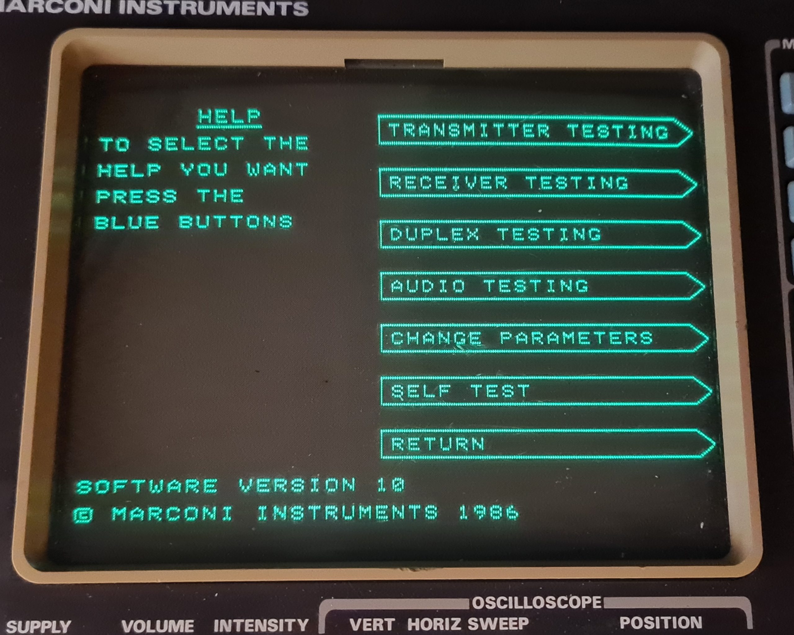
Below, we see the original version 10 firmware, dated 1986.

The EPROMs which need upgrading are IC9, IC10, IC11 & IC12 on the processor board. These are three of 27C128 128kbit (16kByte) EPROMs [IC9-IC11] and one of 27C64 64kbit (8kByte) EPROM [IC12]. I replaced all mine with the larger 128kbit 27C128 parts, copying the 27C64 binary image into both the lower (offset 0x0000) and upper (offset 0x2000) halves of the EPROM, so irrespective of the state of pin A13, the data output would be the same.

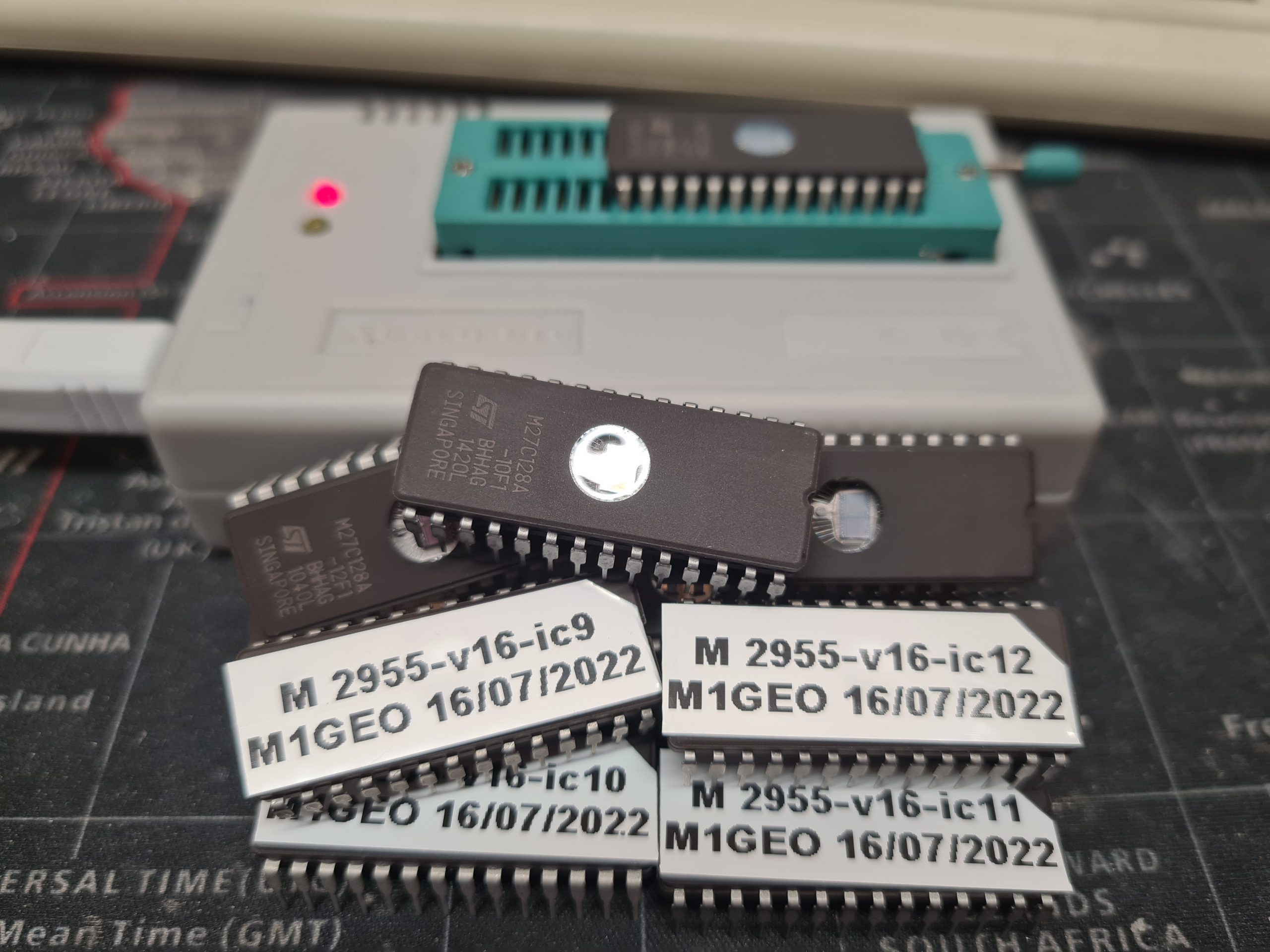
Rather than UV erase the original EPROMs in the machine, I purchased additional ones online (I got mine from AliExpress, but eBay, etc., all sell them). Mine ended up being brand new, never used, but previous ones I’ve bought were pulled from old equipment and needed erasing beforehand.

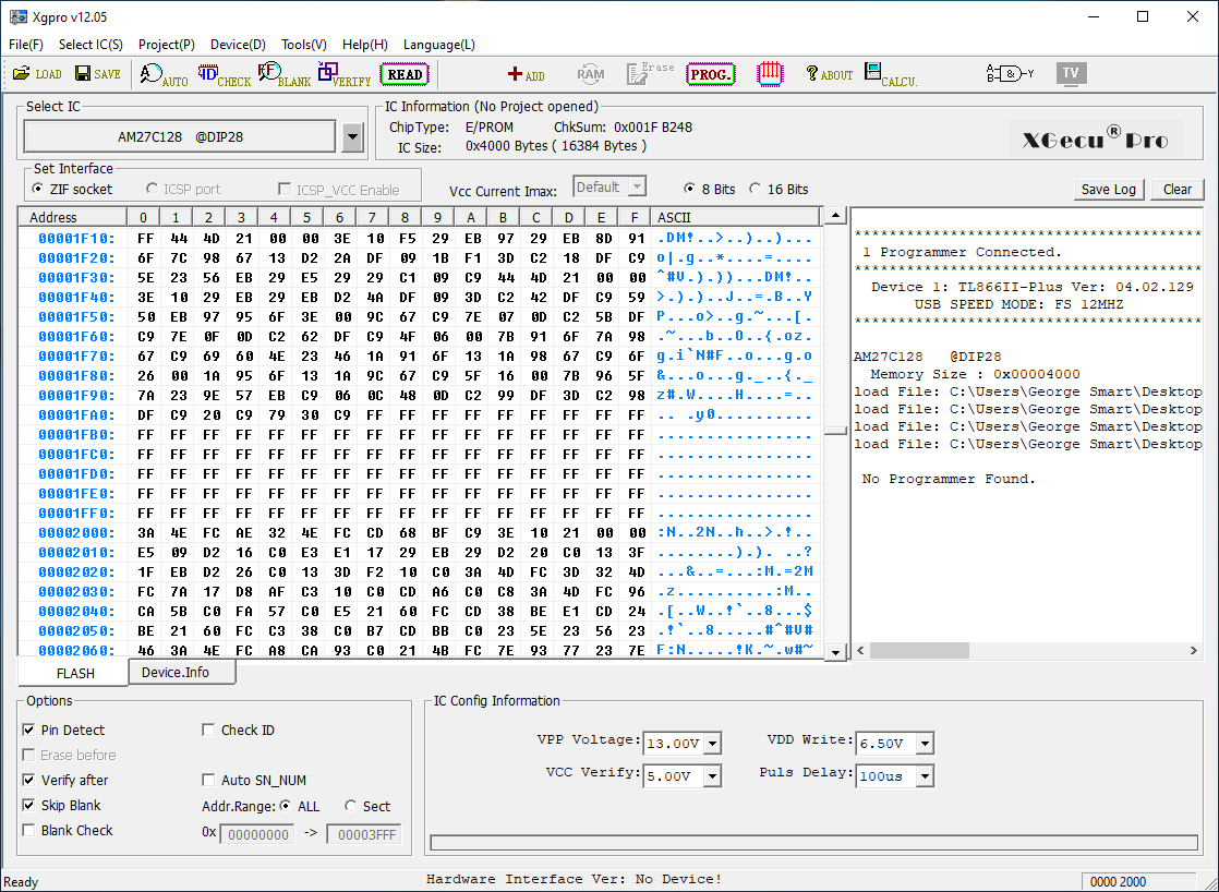
Using an EPROM programmer, I programmed the four 16kB ROMs onto the blank chips. This took around 10 seconds each using my TL866ii+ programmer.

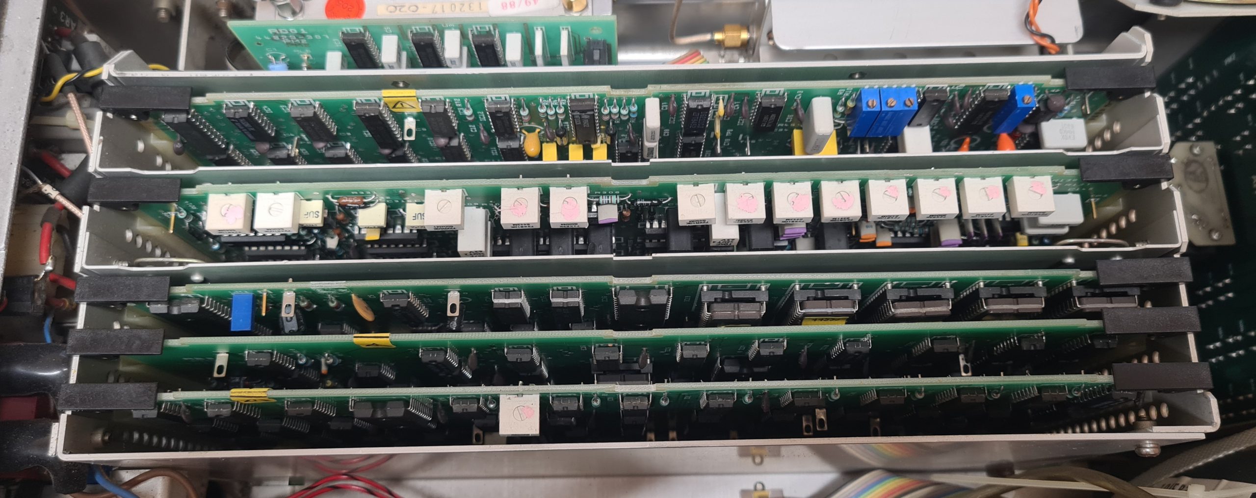
To change the EPROMs in the Marconi 2955, you need to remove the top cover to be greeted with the insides of the 2955. The CPU board (AB4) we need is inside the locked metal cover. These are rotate-clips, not screws, so go easy on them!

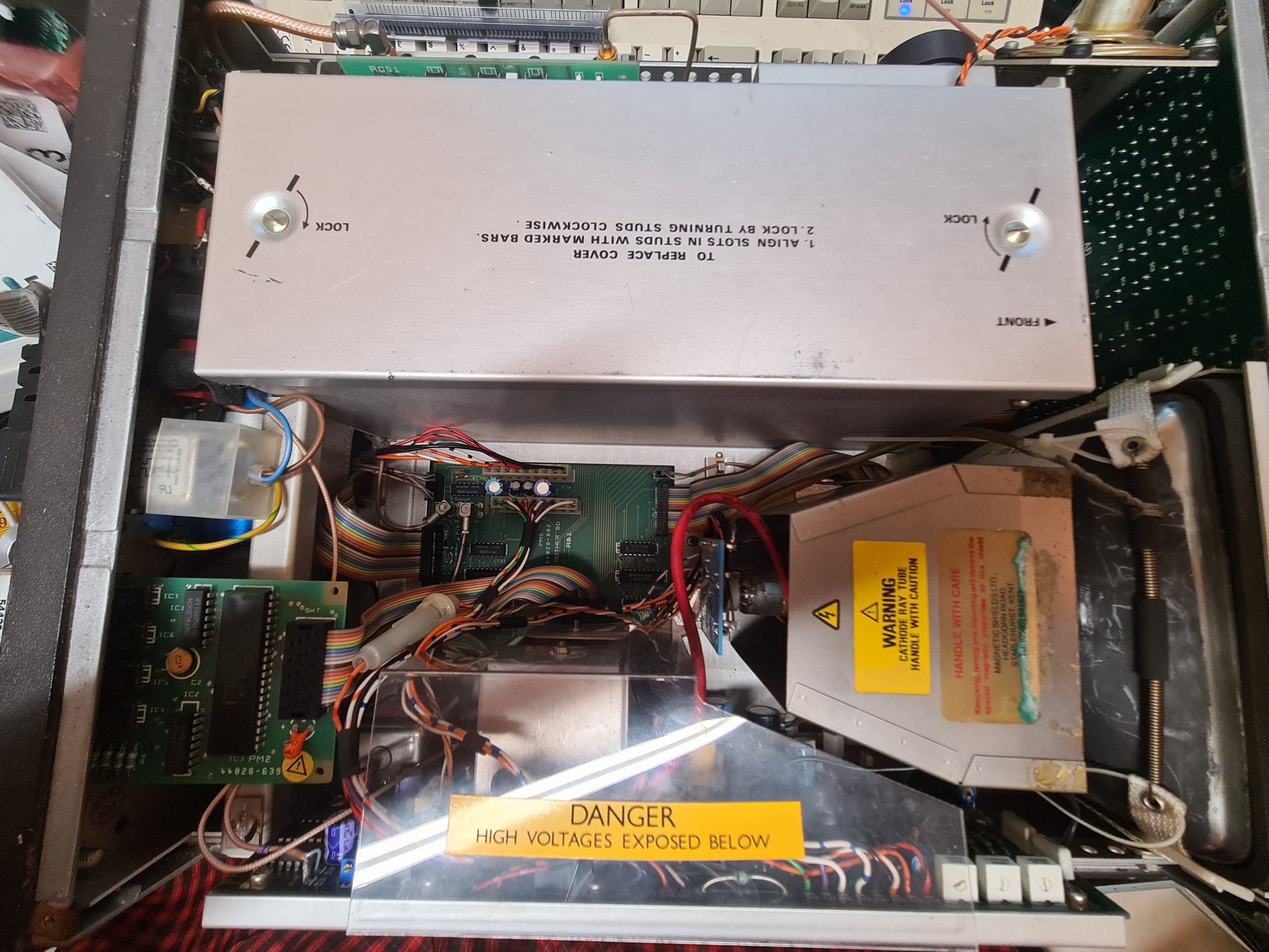
Once you’re inside the metal screening box, you’ll see some boards stacked into the main motherboard along the bottom. We need CPU board AB4, which is the 3rd board up from the bottom of the picture (closest the screen). Use the ‘ears’ on the side to help lever the board from the motherboard socket below and slide the board out.

The CPU board AB4 is shown below. You can see the manufacturer stickers on 3 of the 4 larger EPROMs and the smaller flash EEPROM. From left to right, the 4 stickered devices are IC13, IC12, IC11, IC10 and the final, rightmost is IC9 with missing sticker (it had fallen off inside the machine).

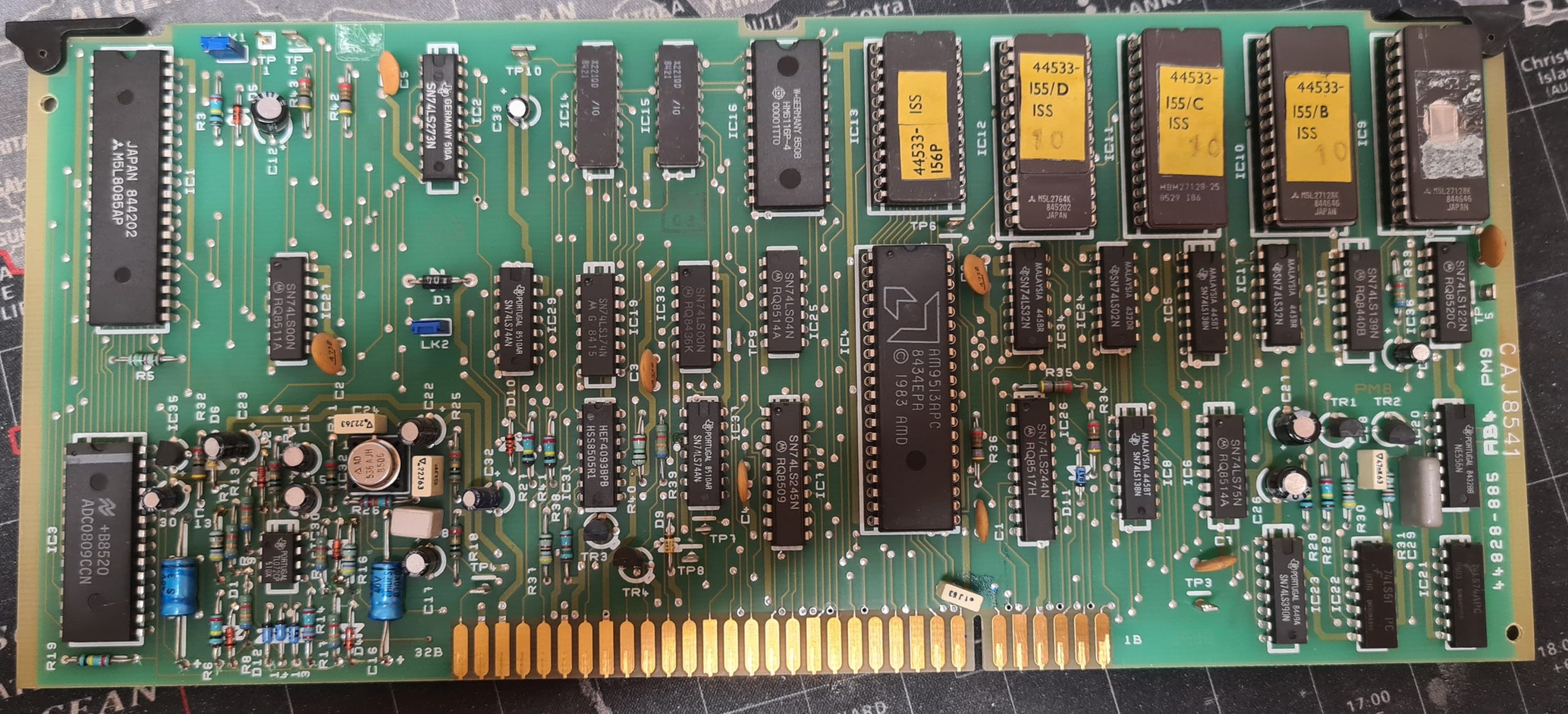
IC13 is a flash chip (Xicor X2816AP) with your unit’s calibration data stored within – don’t overwrite this one any online! You can of course read/back up your calibration data if needed. I decided to copy my flash EEPROM IC13 into a new part, so that I could keep all of my older V10 PROMS together. I was worried that if something went wrong and the V16 firmware had ‘updated’ the formatting of the data in IC13, I may not be able to go back. I used a CSI CAT28C16AP that I had in the shack as I wasn’t originally intending to touch IC13. If you decide to replace IC13 also, I would suggest getting the exact part used in case it matters. These early flash chips are a bit fussy with timings, etc., and so interoperability isn’t guaranteed. That said, mine has been fine.

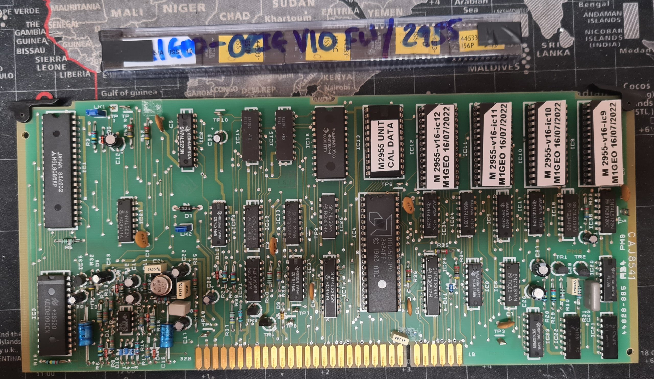
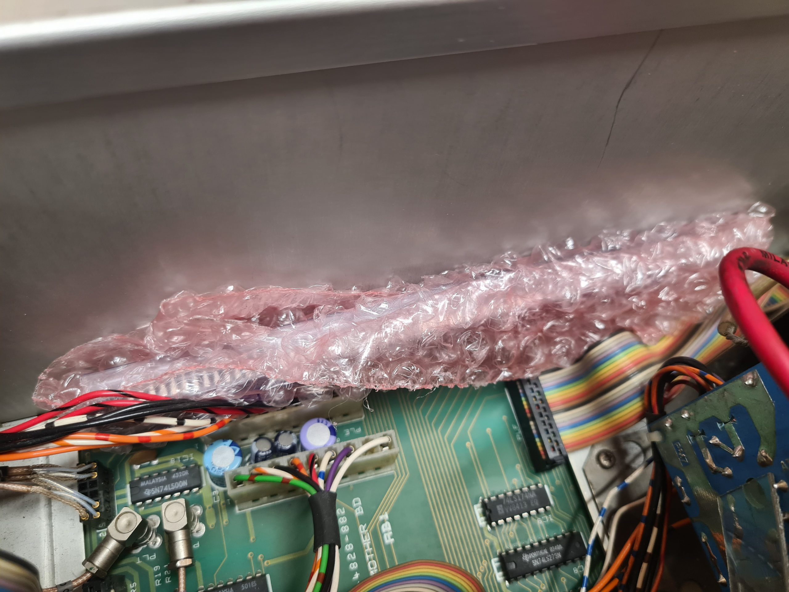
The 5 devices were replaced. I used a label printer to sticker each ROM as I wrote and verified its contents. The original chips were placed inside an antistatic IC tube, and wrapped in ESD-safe bubble-wrap , which I tucked inside the machine between the screened box and the power supply cabling on the motherboard. They sit nicely there, can’t move, and will be available should anyone wish to revert the machine.

After reassembling the unit, I fired the test-set up, and to my relief it booted straight up!

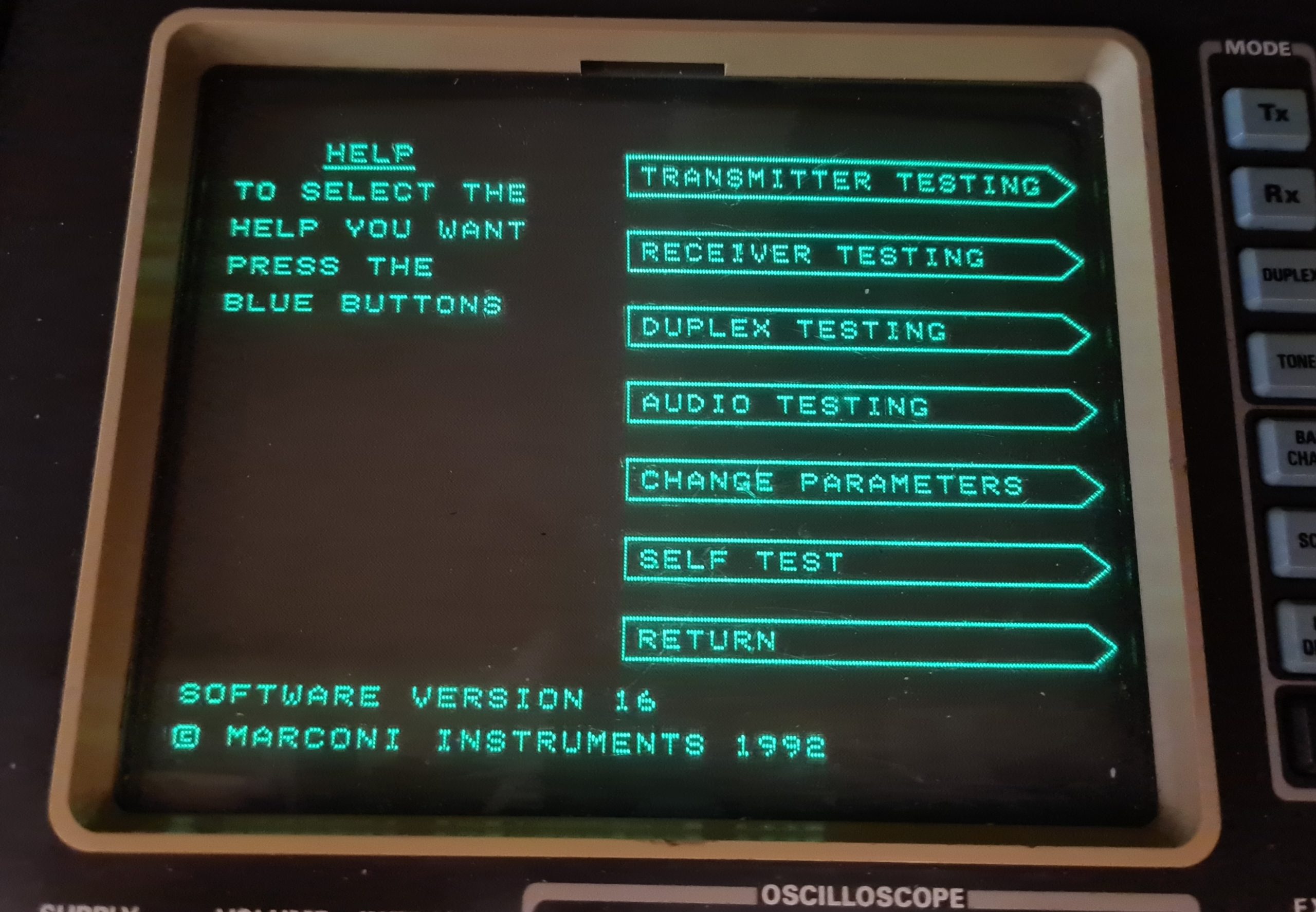
I was able to confirm the firmware upgrade had worked – below we see the software version is now version 16 (dated 1992).

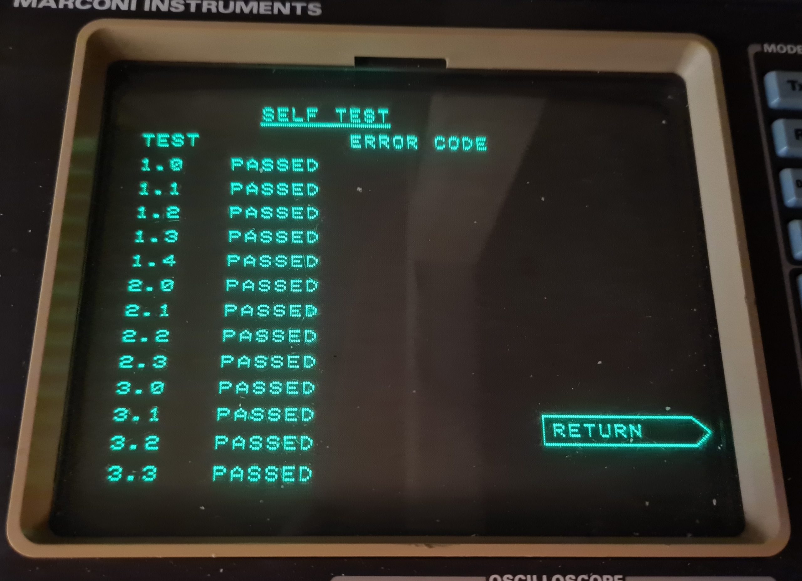
Pressing the self-test button confirmed the basically functional. Excellent!

Symmetricom GPSDO Enclosure

While tinkering with a homebrew GPSDO project, I spent a bit of time searching the depths of the internet for information and parts for my project. I found a PCB for a Symmetricom GPSDO (specifically the Symmetricom 089-03861-02 as per the PCB silkscreen in my case, although the firmware reports itself as 090-03861-03). The board was cheap because the OCXO was missing – I suspect it had aged beyond where the error voltage range was specified, making it unusable. But the board was around £15 GBP delivered from AliExpress, so I took a chance on it based on the fact it had a Furuno GT-8031F GPS receiver which is a GPS module specifically designed for timing applications which “delivers highly accurate GPS timing”. The module also had a CPU (Renesas F2317VTE25V-H8S/2317) with accompanying flash and RAM ICs as well as a Xilinx Spartan-3 FPGA (XC3S200).

Besides the missing OCXO module, my board worked perfectly. I was able to piece most of the information together from the following two resources:

I saw that some people had put their units into Hammond Manufacturing project boxes, and that gave me a few ideas. It would be nice to box the unit up with some ancillary electronics to share the UART (57600 baud, 8N1) over Ethernet TCP/IP. However, my experience of UART to Ethernet modules has always been poor and friends reported similar, so I opted for an FTDI-based USB interface (namely the FT232RL, as the cheapest/easiest part during the chip shortage of 2019-2022). I was tempted to use a Maxim MAX232 device to perform the necessary conversions, but, in the end opted for two NPN transistors – a bit hacky, but much cheaper. I may well come back to the Ethernet option in the future.

The carrier takes 5V at around 2A input on a 2.1mm x 5.5mm DC power socket, a USB-B connector and holds five LEDs: four main LEDs from the GPSDO (which are connected to test-points on the PCB, I can’t find the LED signals on any connector), plus one LED from the FTDI device showing USB activity.

The image below shows where the LED signals are taken from. For reference, the big IC in the centre is the Xilinx Spartan FPGA:

The LED signals are all common anode, fed from +3.3V taken from the board. The LEDs are fed through a resistor, and the individual cathodes connect back to either the CPU or FPGA through another of the wires:

  • RED: +3.3V supply used to power the LED anodes
  • BROWN: Alarm
  • WHITE: Activity
  • YELLOW: Heartbeat (DS2)
  • ORANGE: Error (DS1)

There are two other LED signals (DS3 and DS4) which aren’t connected.

From here, I created a carrier board which had the correct mounting holes for the Symmetricom module, and offered front LEDs to show status, an easy 5V interface and a USB-UART interface to the module control port. The final board looks as below:

With the module fitted, the board looks more like the following. Note, this was an earlier version of the PCB:

The project was designed to fit inside a Hammond Manufacturing 1455N1601BK case which takes a 160mm long by 100mm wide PCB, and the designed PCB fits the case nicely. By default, the Hammond case comes with either aluminum or plastic end plates, but I went to the effort to make PCB front and rear plates to enclose the case. Using PCB meant I was able to use tools I was familiar with to create the end places, and use the same order as the main carrier PCB. The copper on the PCB could be used to create a metal Faraday screen to enclose any electrical switching noise, and the silkscreen could be use to add legends, logos and decals.

I prototyped the designs as below in the PCB package and then used my laser cutter to test them out for fit. A test fit of the front panel is shown below:

The below picture shows the PCB end boards as they arrived and the cardboard cutouts. There are some small tweaks, between the two, but overall the process worked well. One thing to note is that the internal cutouts for the BNC connectors are a little bit tight – in future I need to add an extra 0.5mm or so clearance (in addition to the 0.5mm clearance I left already). However, the connectors pushed in even if a little tightly.

Final assembly went well, and I am very pleased with the results:

An ESP8266 based Air Quality Sensor

Some time ago I had reason to log the quality of air in a room. We needed to know what the levels of carbon monoxide and carbon dioxide were at a given time. I quickly produced a thing on a strip of veroboard that would use an ESP8266 to log over WiFi to the ThingSpeak platform. This proved to be useful, and so I made a couple more on a PCB for various other locations.

The sensor uses a  CCS811 (a low-power digital gas sensor) , BME280 (sensor measuring relative humidity, barometric pressure and ambient temperature) and DHT22 (capacitive humidity sensing digital temperature and humidity) sensors, with an OLED display and a small 5V 40mm fan to waft some air around prior to taking a reading. In reality the project no longer needs the DHT22 sensor, since the BME280 device provides better temperature and humidity measurements and adds air pressure readings. But it is included for historical reasons on my project. Feel free to omit it!

The project is very simple, as it just hooks up modules purchased from eBay. The modules cost less than £2 each at the time of writing and came from eBay or AliExpress.

Since this time, others have asked me for the design files, and so I have now shared them on GitHub: github.com/m1geo/ESP8266-Air-Quality-Sensor. The link contains everything you need to create your own! PCB files, source code and schematic.

If you follow the GitHub link above, you fill find two folders. These are explained in the subsequent sections below.

Code

The code folder contains the Arduino code which runs on the ESP8266 device. You’ll need to source libraries for the SSD1306 OLED, the DHT22 (or cheaper DHT11), the Adafruit BME280 module, and the Adafruit CCS811 module. All these are available inside the Arduino IDE.

The MCU board used is a ESP8266 NodeMCU 1.0. This, and all the modules are easily sourced from the usual places (eBay, AliExpress, etc.), and are cheap. You’ll need to create a ThingSpeak account and then enter your API Key and channel number into the source code, as well as your WiFi name and passcode.

Board

The board folder contains an example schematic design and basic PCB gerber files. You can use these gerber files to have a PCB made. All the cheap PCB houses will produce this board fine. The board files supplied are for the board shown above.

Files

All files are on GitHub: github.com/m1geo/ESP8266-Air-Quality-Sensor

Characterising some VCOs for use in a GPSDO PLL

A key part of a GPS disciplined oscillator is the oscillator itself. During earlier testing I had used two Trimble 34310-T2 OCXO units and one seemed to perform much better than the other. I later read that this may be due to their aging, and that they gradually drift away from their optimal frequency – in this case, 10.000000 MHz – which in turn makes the phase-locked loop (PLL) struggle to converge the frequencies (and thus phase) of the loop. I also have a couple of IsoTemp 143-141 OCXOs, which I will measure, too.

The PLL compares the incoming phase of a reference frequency (here, derived from GPS timings) and the oscillator we’re ‘disciplining’. The loop can work in many ways, but, a common technique is to use digital signals from a phase-frequency detector though an analogue loop filter to generate some kind of voltage control voltage. This voltage is then fed back to the control pin of the oscillator, and the frequency changes accordingly. My post on using a Lattice FPGA development board to create a phase-frequency detector can be found in my Experiments with Phase-Frequency Detectors post.

My first task was to characterise the relationship between frequency and control voltage. For this task, I used a networked spectrum analyser in frequency counter mode and power supply, writing a simple Python3 script to twiddle the control voltage and record the corresponding frequency. I settled on taking an average of 5 readings at each voltage, with the control voltage swept at 100mV intervals through the specified VCO range. I repeated this for each of the oscillators I was hoping to use.

The IsoTemp 143-141 units have a much wider tuning range when compared to the Trimble 34310-T2 modules. In practice this means that the Trimble devices will have greater frequency resolution since they cover a smaller tuning range for the same control voltage range.

Another practical aside is that the IsoTemp 143-141 is a single-ovened oscillator whereas the Trimble 34310-T2 is a double-ovened module. This means that the Trimble unit is much less prone to external thermal variation. However, the IsoTemp unit as a larger tuning range, which will help the PLL keep in lock when there are large temperature variations.

The nominal 10 MHz frequency is found at the following tune voltage for each unit:

OCXO UnitApprox. Tuning Voltage (V)Measured Frequency (Hz)
34310-T2 Old1.9010000000.03
34310-T2 New3.7010000000.04
143-141 #12.1010000000.18
143-141 #22.009999999.78

It is clear from this that “34310-T2 New” is skewed to a higher voltage than the older Trimble unit.

I also observed the warmup time for each of the oscillator modules and the frequency of oscillation without any control voltage applied. Each unit was correctly orientated, supplied with the correct supply voltage as per the datasheet , and without any extra thermal insulation. The room temperature was 21C.

OCXO UnitApproximate Oven Warmup Time (m)Power Requirements (W)Natural Frequency (Hz)
34310-T2 Old~4 (sharp cut off)Max: 8.60
Norm: 2.08
10000000.88
(ΔF: 0.88 Hz)
34310-T2 New~4 (sharp cut off)Max: 8.62
Norm: 2.00
9999996.80
(ΔF: -3.20 Hz)
143-141 #1~5 (more gradual)Max: 2.63
Norm: 1.03
9999999.01
(ΔF: -0.99 Hz)
143-141 #2~5(more gradual)Max: 2.61
Norm: 1.10
9999999.87
(ΔF: -0.13 Hz)

An example of the data captured during the warmup is given below for the Trimble units below:

34310-T2 Old:

34310-T2 New

It is clear to see both Trimble units behave similarly, taking a similar time to warm up at around 4 minutes. The same data was obtained for both IsoTemp modules:

143-141 #1 – I suspect the first point at -1250 Hz is caused by measurement error and can be disregarded. This brings the unit inline with how #2 (below) responds

143-141 #2

The next thing I would like to measure is the phase noise of both of the oscillator units. I have been playing around with scripting the measurement of phase noise of a signal using a spectrum analyser in clever ways. I am able to produce the following graphs. It is important to note that these graphs are not accurate!

A snippet from the IsoTemp 143 datasheet shows these measurements to be considerably distant from the expected results – again confirmation that the above graphs are not accurate.

For now, these are the best I am capable of producing. The numerical values are not absolute, although they should be comparable to those measured on a real noise analyser. However, they’re valid for an optician style “better-or-worse” comparison. I think it is fair to draw the conclusion that the phase noise of the Trimble unit is “better” than that of the IsoTemp unit. It is also worth noting that the output from the IsoTemp unit measured +13.5dBm (square wave), whereas the Trimble unit output only +5.3dBm (sine wave). This extra power required a slightly higher minimum attenuation in order to keep the spectrum analyser happy.

I also took the opportunity to look at the harmonic content for both types of oscillator. First the Trimble unit:

As expected, the IsoTemp produced high levels of odd-harmonics, which is to be expected given the square-wave output:

It seems that both the Trimble and IsoTemp parts are viable in the circuit I have been thinking of. The Trimble has a much more gentle Hz/Volt curve and as a result a smaller adjustment tolerance. Conversely the IsoTemp parts are considerably lower power (6W less, in fact, at peak), and also run at half the power (1W vs 2W) when at temperature.

Watching Propagation with FT8 Spots

Recently I purchased a Hermes Lite 2 SDR receiver (HL2 for short), and I am very impressed with it. One of the very nice features is that it lets you receive several chunks of spectrum (“slices” in SDR parlance) at once.

I also found an excellent piece of software for the digital-mode enthusiast called SparkSDR. SparkSDR can make use of the multiple slices offered by HL2, and thus allows for an infinite number of digital mode receivers to be operated using the HL2 slices. SparkSDR also offers the ability to transmit these modes, but for the purposes of this article, I am only concerned with FT8 reception.

Since FT8 came about, the use of WSPR for making test transmissions and observing receiving locations has pretty much died. However, with the widespread update of FT8 (and similar modes such as FT4, etc.) these transmissions may instead be used as transmitting beacons – when a station calls ‘CQ’ (makes a general call soliciting someone to reply), the software sending the FT8 call encodes the senders location (as a QRA locator) into the sent message. A typical CQ may look something like this:

CQ M1GEO JO02

Similarly, the system of another person responding to my CQ call will also encode the distant station’s location, resulting in a response which may look something like this:

M1GEO ZL1A RF72

Here “M1GEO” is my callsign, “ZL1A” is a DX (distant) station and “JO02” (and “RF72”) is the first part of the maidenhead locator, covering a 100km square, which looks something like this:

It is possible to use a 6-digit locator, for example JO02HG, which takes the accuracy down to a 10km square (see below). Although there are higher resolution locators than this, they are not often used.

Since we know (at least to within 10km) where a transmitting station is, it becomes possible to plot the stations on a map. You’ve probably seen this done before. Websites like PSKReporter and WSPRnet have been doing this for some time now.

The image above use different coloured markers for different bands:

Marker ColourBand
Blue40m (7074 kHz)
Green30m (10136 kHz)
Yellow20m (14070 kHz)
Brown15m (21074 kHz)

I have been recently enjoying the ability to use the same untuned vertical antenna with the same radio on different bands simultaneously (the HL2 lets you remove any band-pass filtering). This allows you to see, for example, that while 40m was good for working Germany, 30m had good propagation into Australia.

PSKReporter lets you filter by mode, band, and time, so you can see what times a given band is open to a specific location. Excellent for helping to fill those missing DXCC slots you may have.

It was interesting for me to see that much of the more remote stations were received on the lower bands, 40 and 30m, and not 20m as I would have expected:

  • VK7BO at 6:06 UTC on 30m
  • VK3ZH at 6:33 UTC on 30m
  • K6SY at 5:28 UTC on 30m
  • LU1WFU at 1:50 UTC on 40m
  • YE8QR at 14:46 UTC on 40m

Although at the time of writing (August 2020), HF conditions are quite poor, not all of the lack of performance on 20m can be explained due to the band conditions, since 20m is still open to South America and into Asia.

Animating the propagation

After looking at these static images, I wanted to see how things changed with time. Could I, for example, see when the best time to work the west cost of the USA would be? I decided to make a time-lapse animation. The animation runs for approximately 3 days, and includes the following FT8 decodes:

BandDecodes
40m (7074 kHz)72,404
30m (10136 kHz)33,871
20m (14070 kHz)156,636
15m (21074 kHz)3,453

It is clear to see sudden bursts of colour when a band opens, and to watch conditions change throughout the day. The dates here were for a Friday to Monday, so, there’s plenty of weekend activity.

I’m keen to further explore the possibilities of this.

Air Particulate Sensor

Background

Around a year ago a colleague mentioned to me the Luftdaten project (en: air data project). It is a sort of citizen science project which measures and records particulate matter in the air. They also have a newer project concerning acoustic noise levels (build notes for this in German here), but I’ll be concentrating on particulate matter here. Often the sensors are combined to collect data on airborne particulate levels, acoustic noise, temperature, humidity and air pressure to name a few. The images below show 24h graphs for some of the measured parameters from various sensors around Europe.

I have long had a fondness for collecting data and the Luftdaten project has plenty! Their website features an interactive map of the world where they plot measurements taken.

The particulates detected include dust, dirt, soot, smoke, and liquid droplets emitted into the air which are small enough to be suspended in the atmosphere. Airborne particulates may be a complex mixture of organic and inorganic substances. The type of sensor used does not differentiate between the particle types, it just gives a measure of how many are present.

Parts

I purchased all of the parts cheaply from AliExpress (no affiliation). You’ll find the same parts on eBay, BangGood, etc., so use what you prefer.

The particulate matter sensor is a Nova SDS011 PM sensor (datasheet), which can be purchased for around £14.

You’ll probably also want a DHT22 temperature & humidity sensor (datasheet) which will cost around £2.

Finally a NodeMCU V3 is required. This is a module based on the ESP8622 WiFi chip, which includes a USB-UART interface, some voltage regulators, etc. In a later step, we’ll program this with the Luftdaten code.

A short length of plastic pipe can help to draw air into the SDS011 sensor. The datasheet for the SDS011 suggests an inside diameter of 6mm and outside diameter of 8mm.

The photo below shows my assembled parts! You’ll notice int he bottom right of the image that I have an Influencair V1.2 PCB. Influencair are a spin-off group of Luftdaten based in Belgium. CivicLabsBelgium produced PCBs for project participants to use and made the PCB Gerber Files available here. You can send these off for manufacture using any PCB service you like (for example, in no order JLCPCB, PCBWay, DirtyPCBs, Elecrow, and so on).

Build notes & Programming

The build process is explained thoroughly on the Luftdaten website under the construction manual page. As I won’t be able to do a better job of explaining this, I suggest you go ahead and read their documentation. Below shows the parts mounted on my Influencair V1.2 PCB. I used 3mm screws to hold everything together.

Programming, Configuration & Registering

The default programming proceedure requires setting up the ESP8622 in the Arduino software environment, but Piotr Dobrowolski has created a very useful tool: airrohr-firmware-flasher for the Luftdaten project. I used the Linux variant of the program the NodeMCU in one click, but Windows and macOS versions exist too! Be sure to find the “releases” button on GitHub to download the pre-compiled ready-to-use binaries!

With the NodeMCU connected to the PC with a USB cable, I selected “latest_en.bin” from the version list (en being English), and pressed Upload. As you can see from the figure below, it took just over 8 seconds and it was done!

Power cycling the board resulted in a WiFi device being created by the newly created sensor! I connected my mobile phone to “airRohr-11189671” and was greeted with the following screen.

I tapped on my house WiFi “SmartLAN”, entered my super-secret passkey and we were away! The device power cycled and was then visible from the flasher once again.

From this, I was able to see the sensor was assigned an IP address on my network, and double-clicking on the entry whisked me off to my default web browser viewing the sensor’s internal webpages.

There are many configuration options, but the defaults were suitable for my hardware configuration. There are options for OLED and LCD screens, extra/different sensors and many other configurations which are out of the scope of this article. However you can click “Current Data” to see the sensors latest measurement data. The image below was taken with the sensor indoors.

The final thing to do is to create an account on the Luftdaten project website so your sensor can contribute measurements. There are already a reasonable number of sensors in the UK contributing data to Luftdaten. You can create your account and submit your sensor data here: https://meine.luftdaten.info

I have positioned my sensor in the garden shed with a short section of plastic pipe poking outside of the shed where the wind blows. I live near a busy roundabout and buy a petrol filling station, so it will be interesting to compare my measurements with other local sensor readings.