Recently I purchased a Hermes Lite 2 SDR receiver (HL2 for short), and I am very impressed with it. One of the very nice features is that it lets you receive several chunks of spectrum (“slices” in SDR parlance) at once.
I also found an excellent piece of software for the digital-mode enthusiast called SparkSDR. SparkSDR can make use of the multiple slices offered by HL2, and thus allows for an infinite number of digital mode receivers to be operated using the HL2 slices. SparkSDR also offers the ability to transmit these modes, but for the purposes of this article, I am only concerned with FT8 reception.
Since FT8 came about, the use of WSPR for making test transmissions and observing receiving locations has pretty much died. However, with the widespread update of FT8 (and similar modes such as FT4, etc.) these transmissions may instead be used as transmitting beacons – when a station calls ‘CQ’ (makes a general call soliciting someone to reply), the software sending the FT8 call encodes the senders location (as a QRA locator) into the sent message. A typical CQ may look something like this:
CQ M1GEO JO02
Similarly, the system of another person responding to my CQ call will also encode the distant station’s location, resulting in a response which may look something like this:
M1GEO ZL1A RF72
Here “M1GEO” is my callsign, “ZL1A” is a DX (distant) station and “JO02” (and “RF72”) is the first part of the maidenhead locator, covering a 100km square, which looks something like this:
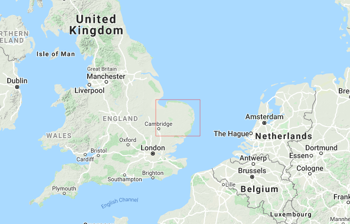
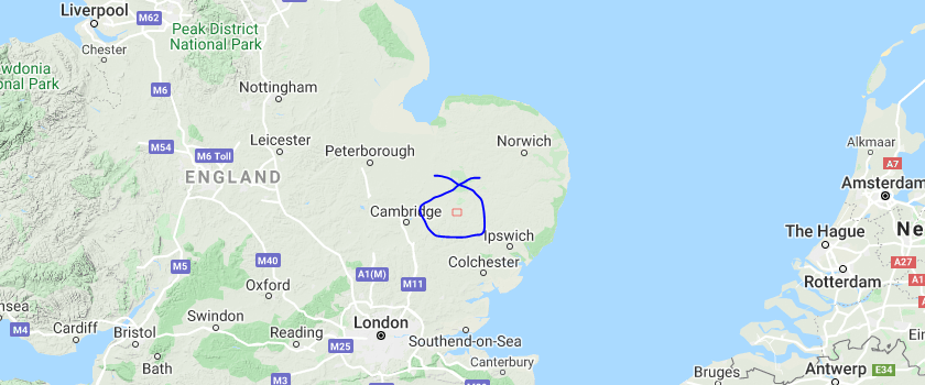
It is possible to use a 6-digit locator, for example JO02HG, which takes the accuracy down to a 10km square (see below). Although there are higher resolution locators than this, they are not often used.
Since we know (at least to within 10km) where a transmitting station is, it becomes possible to plot the stations on a map. You’ve probably seen this done before. Websites like PSKReporter and WSPRnet have been doing this for some time now.
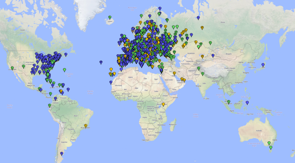
The image above use different coloured markers for different bands:
| Marker Colour | Band |
| Blue | 40m (7074 kHz) |
| Green | 30m (10136 kHz) |
| Yellow | 20m (14070 kHz) |
| Brown | 15m (21074 kHz) |
I have been recently enjoying the ability to use the same untuned vertical antenna with the same radio on different bands simultaneously (the HL2 lets you remove any band-pass filtering). This allows you to see, for example, that while 40m was good for working Germany, 30m had good propagation into Australia.
PSKReporter lets you filter by mode, band, and time, so you can see what times a given band is open to a specific location. Excellent for helping to fill those missing DXCC slots you may have.
It was interesting for me to see that much of the more remote stations were received on the lower bands, 40 and 30m, and not 20m as I would have expected:
- VK7BO at 6:06 UTC on 30m
- VK3ZH at 6:33 UTC on 30m
- K6SY at 5:28 UTC on 30m
- LU1WFU at 1:50 UTC on 40m
- YE8QR at 14:46 UTC on 40m
Although at the time of writing (August 2020), HF conditions are quite poor, not all of the lack of performance on 20m can be explained due to the band conditions, since 20m is still open to South America and into Asia.
Animating the propagation
After looking at these static images, I wanted to see how things changed with time. Could I, for example, see when the best time to work the west cost of the USA would be? I decided to make a time-lapse animation. The animation runs for approximately 3 days, and includes the following FT8 decodes:
| Band | Decodes |
| 40m (7074 kHz) | 72,404 |
| 30m (10136 kHz) | 33,871 |
| 20m (14070 kHz) | 156,636 |
| 15m (21074 kHz) | 3,453 |
It is clear to see sudden bursts of colour when a band opens, and to watch conditions change throughout the day. The dates here were for a Friday to Monday, so, there’s plenty of weekend activity.
I’m keen to further explore the possibilities of this.