
Recently, while trying to track the signal strengths of radio beacons I encountered a difficult problem: getting an accurate and high-resolution measurement of signal strength. Using my Yaesu FT-857D and the Yaesu CAT Interface I tried to sample the S-meter (using rigctl via the get_level command and requesting STRENGTH, if you’re interested). This didn’t work very well as the S-meter readings were very low resolution and that the pass-band of the radio is too high (the signal is hard to track in noise).
While talking to Dave Mills (G7UVW) regarding the issue, he suggested a digital signal processing approach. I immediately thought of my Third Year Project work and decided to conduct a few experiments.
Proof of Concept
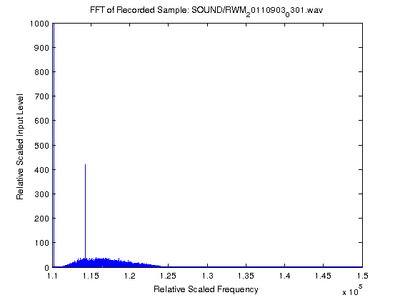
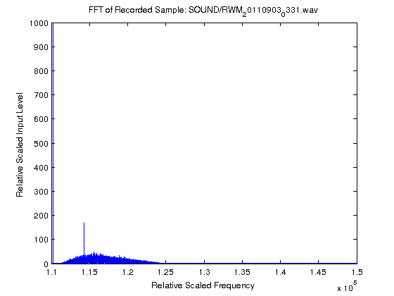
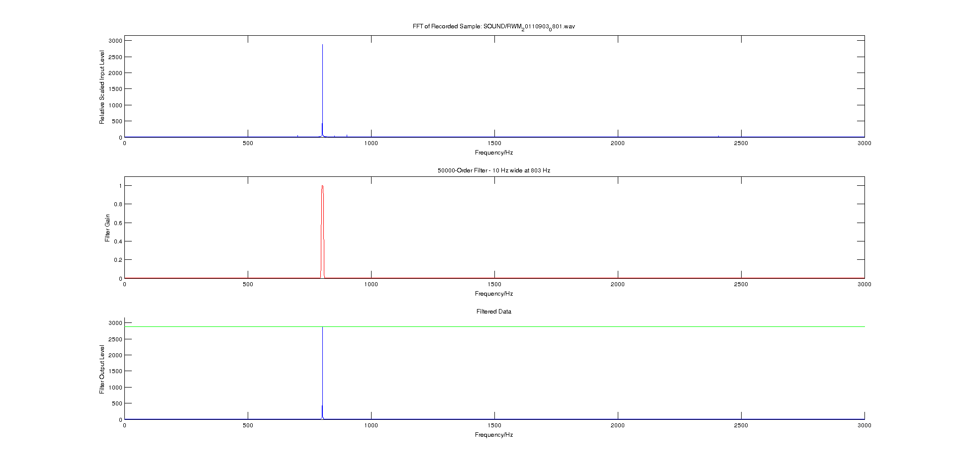
The two graphs below show the very first results, acting of a “proof of concept” more than anything else. 5 seconds of audio was recorded from the radios’s audio output and analysed via FFT in MATLAB. As you can see, the approach showed promise.
 |
 |
Click an image to get more information, or twice to enlarge fully.
In the images above, the very large spike right next to the Y-axis is DC. The smaller spike is the 800Hz signal. The grass along the bottom is the shape of the Yaesu FT-857D‘s CW filter. The two graphs are scaled exactly the same and so the size of the spike makes for a direct vertical comparison. The left most image shows the FFT analysis when the received signal was about S9 on the meter. The right image shows when the received signal was below the noise floor. However the noise floor was S8 at the time of experimentation, and so it reflects on the coherent and continuous nature of the tone versus the random properties of the noise when the two signals are analysed coherently (as is inherent here).
Scaling the Graphs
The graphs above are not scaled. The X-axis values have an complex mapping to the frequency domain which they represent. This section details how I went about getting from these values to values in Hz. The key is the sample-rate in the time-domain, which sets the resolution (bin-size) of the FFT. Engineering Mathematics by A. Croft et al. (ISBN:0130268585) includes some excellent examples of how this works.
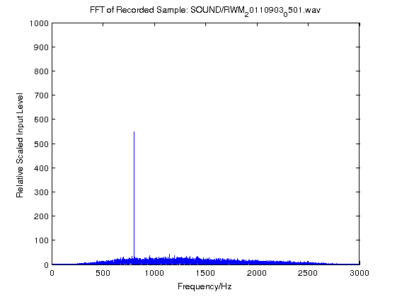
In simple terms, the sample rate in the time domain transforms to the frequency in the Fourier (frequency) domain. Here we’ve a sample rate of 44100 Hz, and so we get a frequency range of -22050 to +22050 Hz. The frequency scale essentially runs from -SampleRate/2 to +SampleRate/2. The negative frequency range is useful for retaining phase information but is essentially a mirror image of the positive frequency region. We create a vector based on the parameters of the input file and plot our FFT data against it. The end result is to have a scaled frequency axis. The graph below shows this. Note that the frequency domain goes on until 22050 Hz, but the radio passband is only 3000 Hz wide and so we cut the graph there.
Digital Filtering
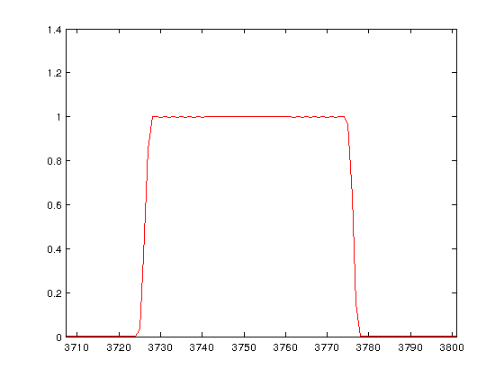
In order to remove the DC and much of the noise, we can create a sharp filter around the 800 Hz signal we want. Simple reasoning would have us simply create a vector of zeros say for the sample corresponding to the 800 Hz signal, which has a value of one. Multiplying this vector with our FFT data would essentially filter out only the 800 Hz signal. This is what we do… Kind of! Having a square window causes noise in the passband, due to concepts beyond the scope of this page and is not usually recommended. Other shapes or windows exist that avoid this problem. They are essentially variations on the square window (often called the brick-wall filter) which have specific noise characteristics. See the Wikipedia: Window Function article, specifically the examples part for more on this. Here we will use the Hamming window to create a linear-phase filter with normalized bass-band gain. The filter shape looks something like the following:
The process of filtering the input signal through the above filter is to just multiply each element in our original FFT data by the corresponding element in the Hamming-window vector. The image below shows the process flow, going downwards, from getting the raw FFT, creating a filter, and finally filtering the data through the FIR filter. The image below is high-resolution, so click on it twice to get the full high-res image.
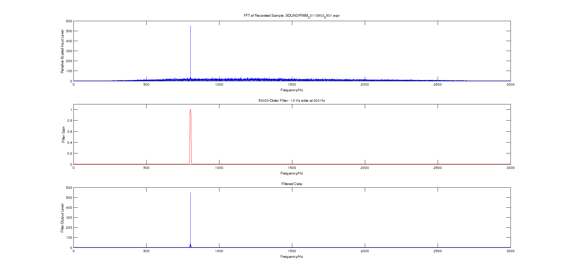
Once properly implemented, the filter option takes parameters such as centre frequency, bandwidth and order. In simple these parameters allow for a tight fit of the signal.
Obtaining an RSSI
An RSSI (receive signal strength indicator) is a numerical value relating to the amount of power present in a received radio signal. This value is ultimately what I need to compare the strengths of beacons. Calibrating this is somewhat meaningless for my application and as a result the values obtained will be related by the same arbitrary (unknown) constant.
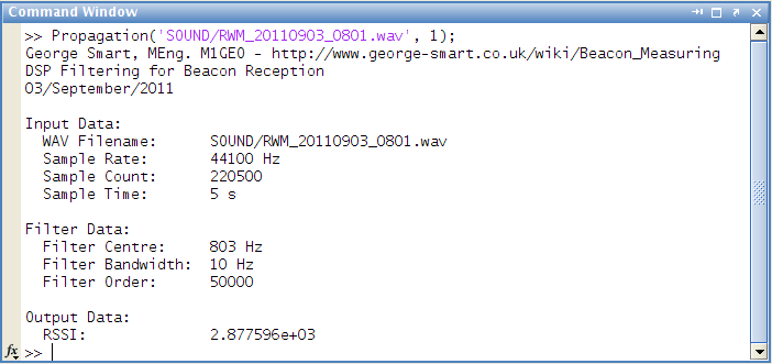
This can be done by taking the maximum value of the filtered data, i.e. the peak of the bottom graph. A small piece of code is added to draw a line across the bottom graph (in green) which is the RSSI value.
The program is also modified to output the RSSI value to the calling window in MATLAB, and return the RSSI as the method’s return value (suppressed in the below image, with the semicolon on the calling statement).
Automation
To get a data for a nice looking, well sampled graph, it is obviously necessary to collect a large number of RSSI reports. This would be a laborious process, as previously the MATLAB script required me to already have sampled the radio’s output into a wav file. I wanted something that I could leave running for a week or so and collect data automatically, hence the need to automate the process. I wanted to avoid having weeks worth of wav files on the computer’s disc drives as this would use a lot of space. So I set about modifying the MATLAB script again to accommodate these needs.
The AudioSample.m file opens the computer’s sound card, and passes a recording object to the CalculateRSSI.m script (based on the earlier Propagation.m file). This enables the CalculateRSSI.m function to sample the soundcard automatically and simply return a numerical value for RSSI. This value is then logged, along with the timestamp by AudioSample.m. The program is now just two MATLAB scripts and everything is done from within MATLAB. There is no need for external sampling. The system will plot pseudo-real-time graphs, as the following YouTube video shows (HD is probably preferable here, to read text).
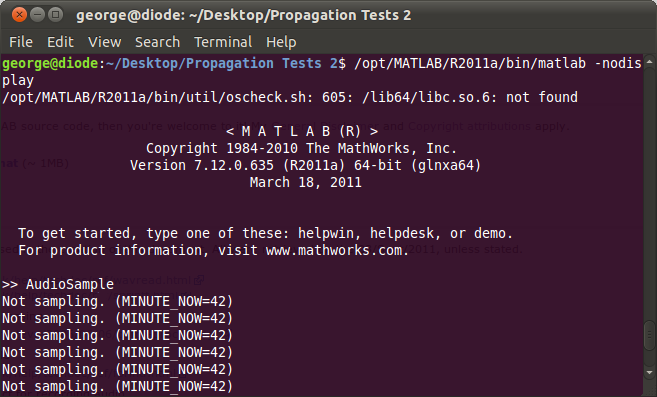
The errors presented are minor glitches and do not stop the program from running.
Plotting
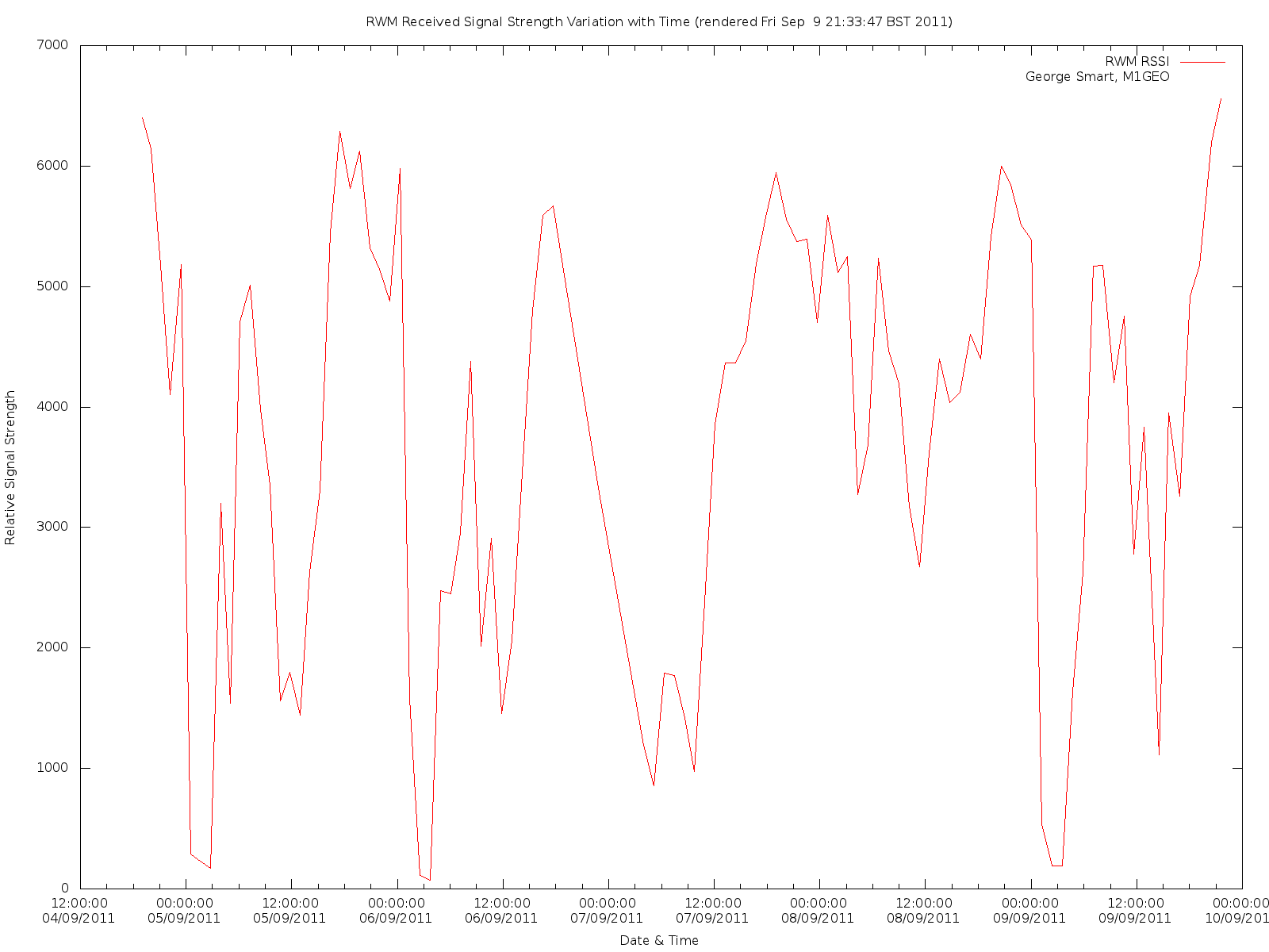
From the CSV output by MATLAB, it is then possible to perform some statistical analysis on the RSSI data obtained. The first step was to plot an averaged version of the RSSI change as a function of time. This is what the image below shows.
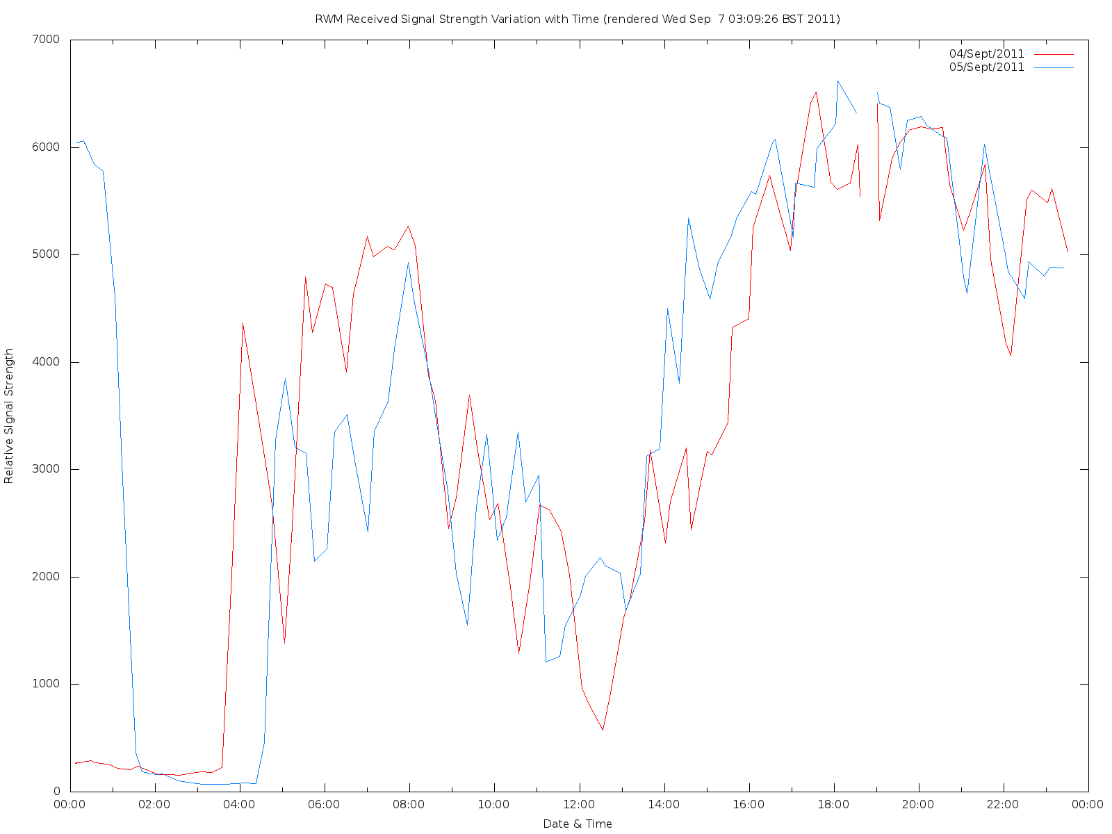
After collecting data for a couple of days, it occurred to me that there were patterns in the RSSI readings; these turned out to have a period of about a day. Here the below graph shows the RSSI readings for two consecutive days, the 4th and 5th of September, 2011. The gap around 7 pm is where the recording MATLAB script was stopped, edited, and relaunched to make a slight alteration to functionality. It should be noted that the graph want’s to wrap around from end-to-end – although these lines have been removed for the sake of tidiness, there are indeed lines linking the right-hand with the left hand to complete the loop.
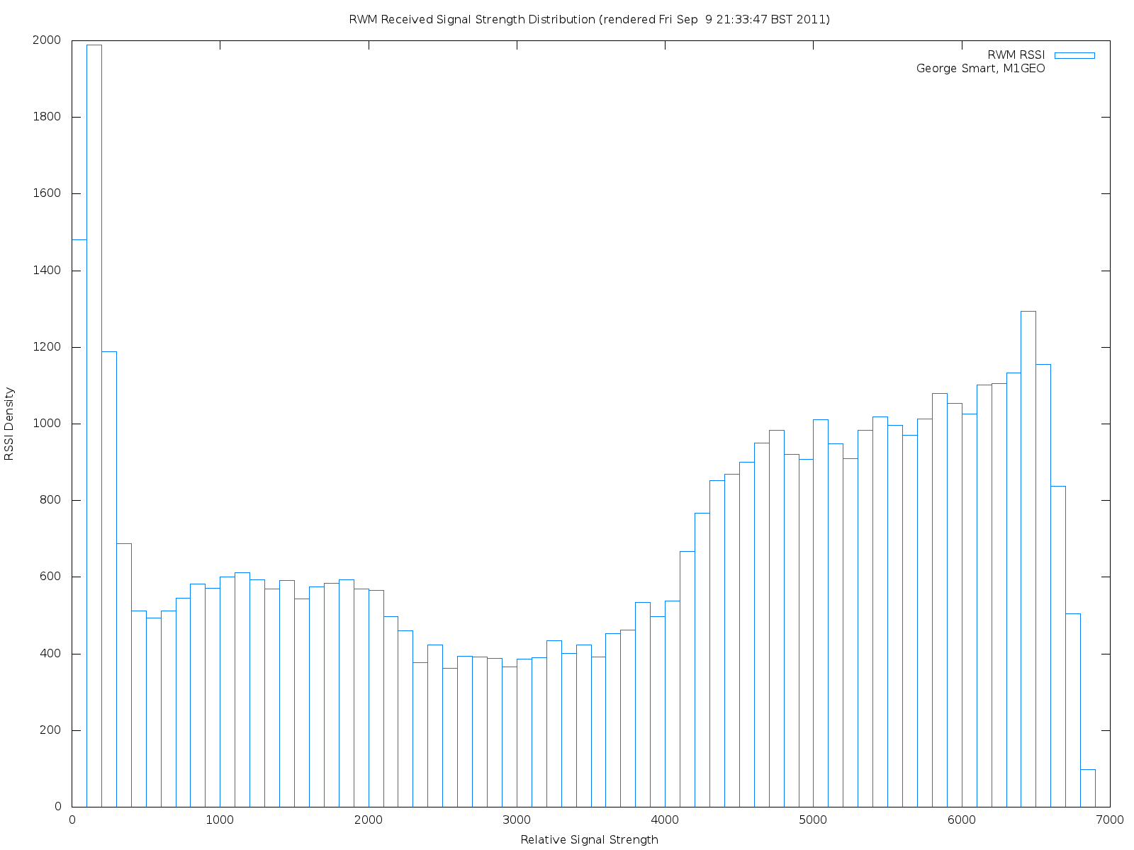
Next off I decided to have a look at how the RSSI is distributed. The next plot shows the distribution of RSSI amongst the possible values.
Download
If you’re interested in the MATLAB source code, then you’re welcome to it! This file includes two MATLAB files and two gnuplot files.
*** Source Code in Tar-Gzip Format *** (~ 2KB)
My General Disclaimer and Copyright attributions apply.