Over the past few years I seemed to have amassed a vast number of antennas, all of which were stored on the workshop roof. Recently when looking for a 2 metre beam I found I had two beams on the roof. A quick measurement with the MFJ Antenna Analyser revealed these antennas were either broken completely or tuned for the American 2-metre band, centring on about 146MHz. I intended to use my beam for 2-metre SSB and so a frequency of 144.3MHz was required. I decided to go about designing a new antenna for the frequency required both to learn about antennas and to end up with an antenna meeting my needs. I had enough parts and pieces of metal lying about, so I figured why not have a go. This page documents the design, making and testing of this antenna.

I have also made a 432MHz Yagi, which you may also be interested in.

Designing

The Yagi was designed using Martin Meserve’s VHF/UHF Yagi Antenna Design tools.

The beam was designed for a resonant frequency of 144.3000 MHz at a drive impedance of 50R. This is typical for 2-metre SSB operation and is nicely compatible with my Yaesu FT-857D that I use for portable operation. A target gain of 7 dBd was used to keep the beam a small size, although in theory the beam made calculates to 8.2 dBd. It has 1 reflector, 1 driven and 4 director elements. ARRL standards were adopted for reflector and element spacing, with all elements having an outer diameter of 9 mm. A boom diameter of 32 mm was used, due to me already having it. The design shown below is for a bonded beam, meaning the elements are electrically connected to the boom at the element centre.

The image below shows the design of the beam, and contains both the element length and cumulative spacing – everything you need to have ago!

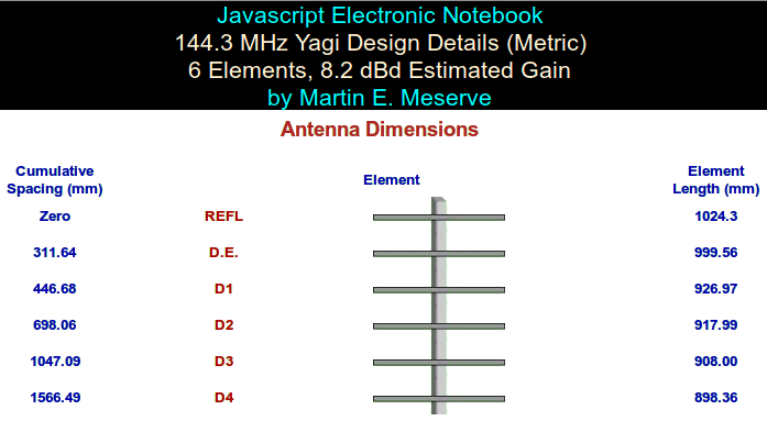
Note that this diagram is not to scale.

Specifications

Frequency	Gain	Horizontal B.W	Vertical B.W	Electrical Boom Length	Boom Diameter	Element Diameter	Dimensional Tolerance
144.3 MHz	8.243 dBd (10.393 dBi)	49.9°	55.1°	1605 mm	32 mm	9 mm	6.2 mm

B.W = beam width. Boom must be at least the electrical boom length long.

Making

Dimensions Table

	REFL	Driver	Director 1	Director 2	Director 3	Director 4
Element Length (mm)	1024.3	999.56	926.97	917.99	908.00	898.36
Cumulative Spacing (mm)	0	311.64	446.68	698.06	1047.09	1566.49

Making the beam was fairly straight forward. I marked two lines down the boom, one on each side, exactly opposite each other. Mark the position of the reflector (REFL on the above diagram). This is the reference of zero – everything else is measured along this line with respect to the reflector. From this, measure the other element locations, marking them out based on the dimensions table, above. Then repeat this on the other side of the boom. Drill the holes required to fit your chosen size bolts – care should be taken that the size of hole does not weaken the smaller diameter elements.

Cut the elements to length as specified in the dimensions table, above. Also mark the centre of each element as you will need to drill a hole there to fix the beam to the boom. Once you’ve drilled the cut elements, go ahead and fix them to the boom. Your beam should have taken shape, and at least look like an antenna… Now to get some RF into it!

Gamma Matching

A gamma matching section provides a way to drive the antenna at the correct place and present the correct impedance to the RF source. There are many ways to achieve this, and many of these ways are suitable here; however, I chose the gamma match as it is well suited to the Yagi – it is physically simple to create and calibration is straight forward. It is cheap too, and requires few parts!

Gamma Match Design

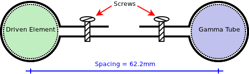
Alan, VE3SQB has written a great program for designing gamma matches. The image below is the design suitable for our antenna created by his software – it is very simple to use!

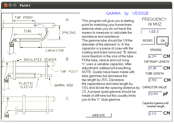
I’ve opted for method B. This uses a thicker coax’s centre to make a capacitor. I used some RG213. Taking the centre conductor and dielectric, and inserting it into a section of 9 mm tube creates a capacitor. The coax centre is soldered to the hot pin of the SO239. The tube over the dielectric becomes our gamma rod. This is connected by a clamp to the driven element. The clamp is fixed to the driven rod at the tap point as calculated by the program above. The capacitance is then adjusted by moving the gamma rod to cover the coax dielectric more (increased capacitance) or less (decreased capacitance). If this sounds a little complicated, I hope the diagram below and the picture of my gamma match will help clarify.

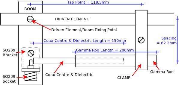
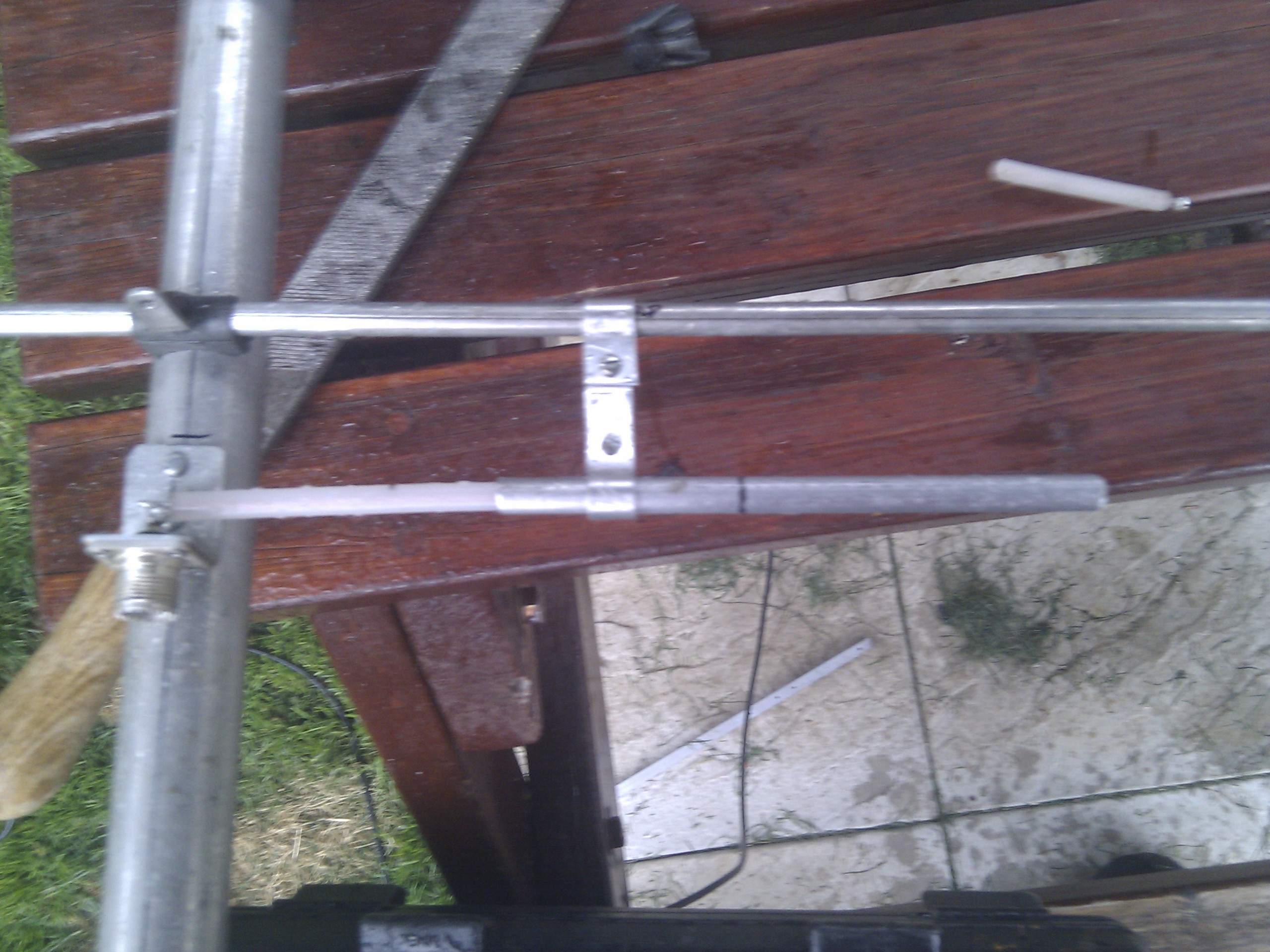
I’ve opted to mount my gamma network on the right side of the antenna, as it seemed most natural. A small piece of folded aluminium is used to hold the SO239 connector. You can see that the placement of the SO239 connector depends on the spacing between the driven element and the gamma rod. Here the spacing is 62.2 mm, as specified by the software above. The coax centre soldered to the SO239 hot pin is then aligned to give the required spacing. The SO239 socket is then mounted on the boom, ensuring an electrical connection between the ground of the SO239 and the boom.

The tap point is located 118.3 mm from the boom/driven element fixing. This is where the clamp meets the driven element. The value given is a suggestion as a starting point – this is of course an adjustment for the antenna. A clamp where it is possible to adjust grip on both tubes independently allows for much easier adjustment. I folded a strip of aluminium as follows:

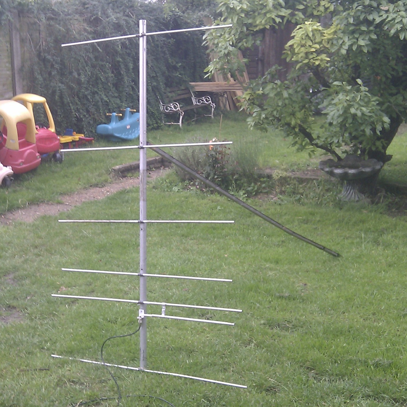
The Antenna

The image below is of the completed Yagi, end up. Note here that the gamma tube is longer than the design specifies. This was before calibration of the antenna occurred; I wanted to be sure not to unnecessarily cut the tube.

Calibration

Calibration is pretty simple. Starting with the clamp at the default tap point, ensure that the clamp is tight on the driven element. Then adjust the gamma capacitance by moving the gamma tube to exposing more or less of the coax centre dielectric. This should be adjusted for the lowest SWR at the desired frequency. This can be done using a Vector Network Analyser, an Antenna Analyser, or by means of radio and SWR bridge. Start with minimal capacitance (minimal overlap) and gradually increase the overlap by pushing the gamma tube over the coax dielectric. You should notice a dip in SWR. If the SWR dip isn’t low enough for your application, then try adjusting the driven element tapping point; you will need to re-adjust the capacitance afterwards, however.

As general rules;

The driven element length sets the resonant frequency
The driven element tapping point sets the feed impedance
The gamma capacitance offsets the inductance bought about by the tapping offset, and so alters the SWR of the antenna.

These rules are just guidelines, and in reality all factors are interlinked.

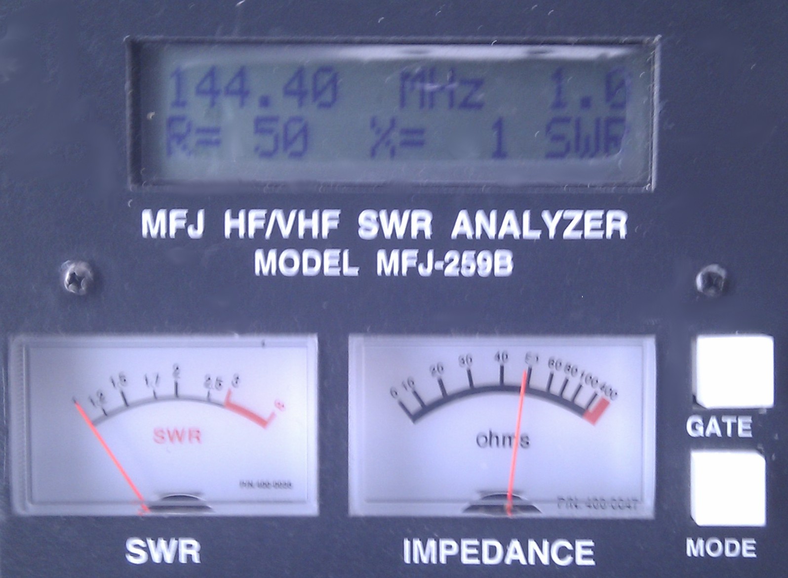
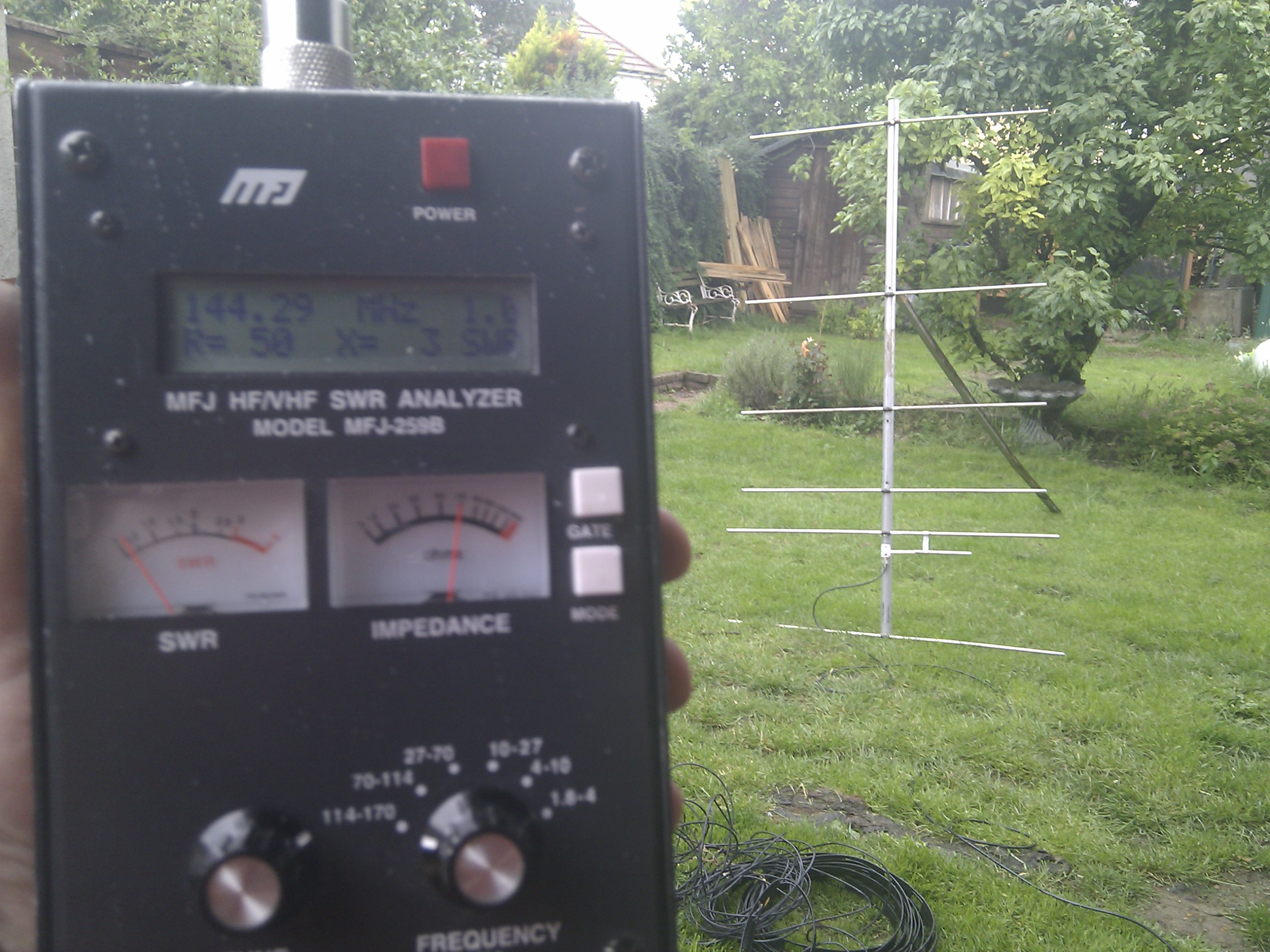
From the antenna analyser, we see that the antenna is a near perfect match at 144.4 MHz, with an SWR of very close to unity (1-to-1) and a drive impedance of 50R. Exactly what I wanted!

Testing

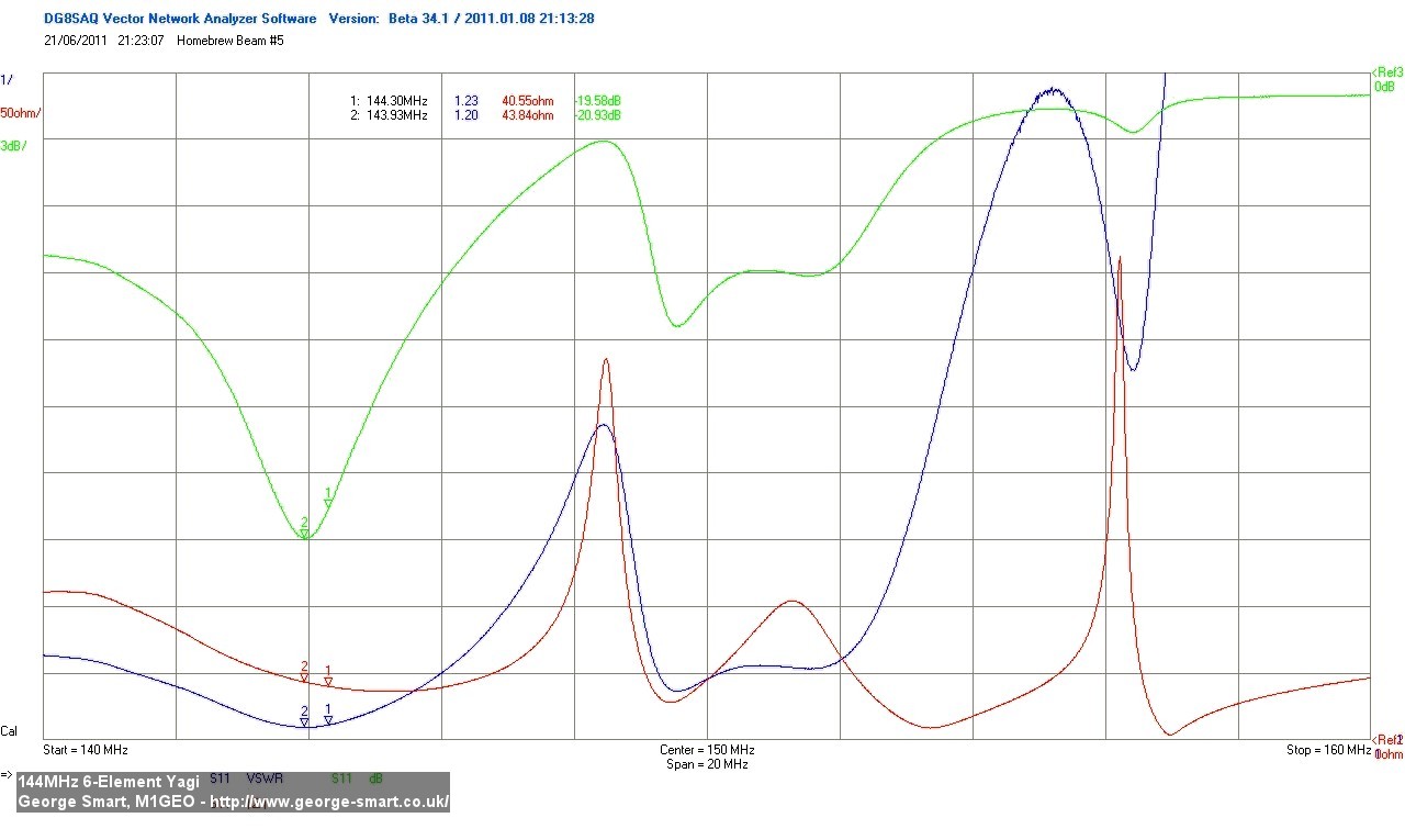
Once the antenna measured up well on the antenna analyser, I connected it to the vector network analyser for a more detailed and in depth look at its functionality. These are based on S11 (reflection) measurements of the antenna – i.e. looking at the reflected power from the antenna. The JPEG compression on these images has lost the colour contrast. Be aware that both the horizontal and vertical scales change between some images.

This first graph shows the VSWR, feed impedance and antenna reflection gain as a function of frequency. On this graph, the frequency was swept from 140 to 160 MHz and the antenna measured. The blue trace shows the SWR, the red trace shows the feed impedance, and the green trace shows the ‘antenna’s loss’ (radiated power shows up as a loss in reflected power – the energy is lost in transmission and not reflected back). The bottom line serves as a reference for VSWR (representing a perfect match, 1:1) and for drive impedance (representing 0R feed impedance). The VSWR scale increases linearly vertically once per division. The feed impedance increases in intervals of 50R per linear vertical division. Finally, the dB loss graph (green trace) serves no quantitative purpose other than to show the sharpness of the antenna response.

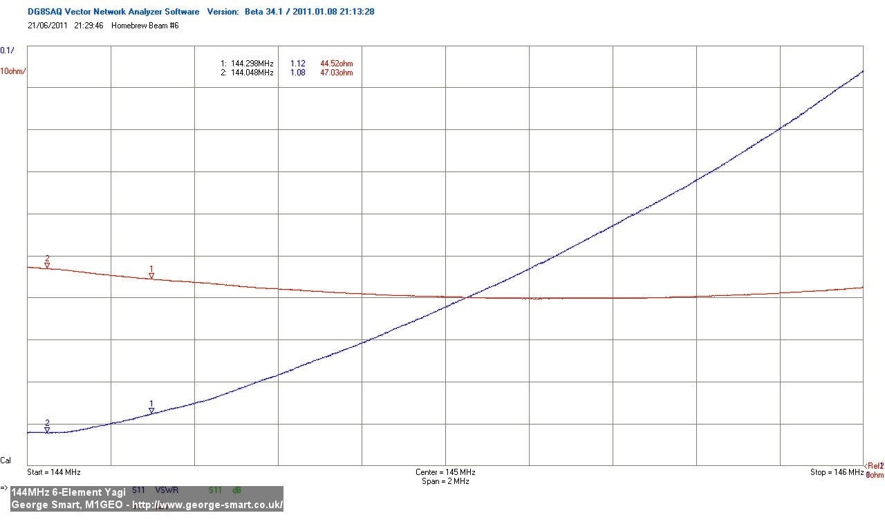
This graph again shows VSWR (blue trace) and feed impedance (red trace). Here the VSWR scale increases in divisions of 0.1, and the feed impedance remains 50R per interval. We see that at the two markers ([1] 144.3 and [2] 144.05) the VSWR is 1.12:1 and 1.08:1 which are respectable values. The graph serves to show that the antenna behaves well over the UK 2-metre band (144-146 MHz) of interest. The VSWR fluctuates very slightly, and the feed impedance wobbles slightly around the 50R mark, which is ideal for my requirements.

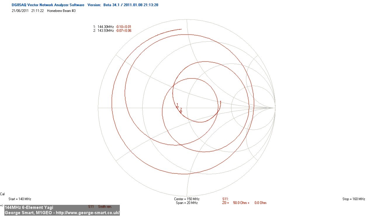
The Smith Chart shows a lot of information about the antenna. Marker 1 shows the point at which the antenna is used, and shows that the antenna is a resistive load (on the bisecting line through the chart).

Co-axial Cable

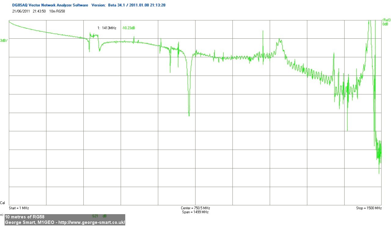
I decided also to examine the loss of the cable I was using to link the antenna and VNA. It is important to note that the graphs above were plotted in such a way as to eliminate the effects of the coax. However, I was interested in how coax responded at various frequencies. I performed an S21 (through power loss) test on 10 metres of brand new RG58.

The top of the graph is normalised to a reference of 0 dB. Each division represents a loss of 3 dB.