With Parks on the Air (POTA) becoming a relatively new thing in the UK, I decided to activate a few local parks. It quickly became apparent that many of the local parks had never been activated before. I decided that I would concentrate on those.
I suspect that they hadn’t been activated before because they required a bit of a walk to get to. What with it being winter and wanting to get out of the house, I kitted up my backpack with my Icom IC-705, my EcoWorthy 8Ah LiFePo4 battery (see my notes on IC705 power vs voltage) and a few antenna options. Over the course of a few evenings, heading to a different park each night after work, I activated the parks I had seen on the POTA App Map. I wanted a way to find any parks that were local, but that hadn’t been activated.
With services like SOTL.AS for Summits on the Air (SOTA), it’s easy to filter the map to only show specific things, like removing summits you’ve activated, or setting a minimum number of activator points, or showing only summits that haven’t been activated before. Unfortunately no such service exists for POTA (yet). If you’re reading this and considering doing something similar, check out SOTLAS first 🙂
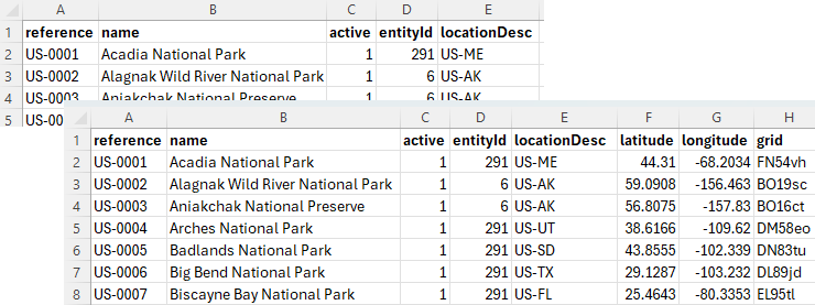
The POTA website does offer all_parks.csv (list of all POTAs) and all_parks_ext.csv (list of all POTAs with location information). However, neither of these files have the information I was looking for: the number of activations or attempted activations. Disappointing, but I didn’t give up that easily! I did some digging!
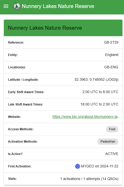
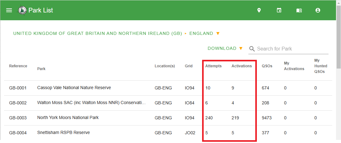
By searching the POTA ParkList for parks in my country, in my case “GB-ENG”, I was able to see the information I needed. At this stage, you could just sort the columns by activations, and skim through looking for close places. However, I wanted to do better than that! I wanted to create a program that would list them by how close they were to me.
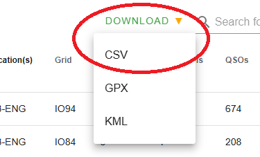
The observant amongst us will have noticed the “DOWNLOAD” button, that yields a CSV file for us. You may have to be logged in to see this, as it contains information personal to you (your activations, and hunts). I missed this the first time and subsequently copied and pasted the information manually from the webpage into a spreadsheet and exported it to a CSV which took about 5 minutes!
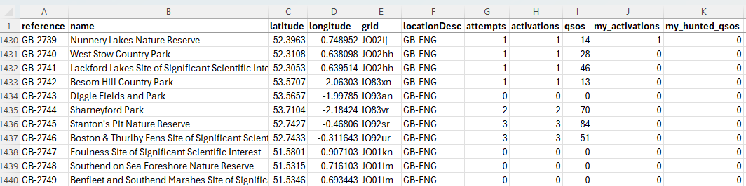
Regardless of how you chose to obtain the information, you’ll end up with a CSV file. Mine was called “England.csv”. The data inside is really useful and includes the latitude and longitude of each marker. Any program would just need to work out how far each site is from a given location (say, your home QTH) and then sort the output by distance. It could filter on attempts or activations, too.
The Program
So I set about writing a simple Python program (really more of a script) that lets you explore your POTA CSV file and (most importantly for me) find the closest unactivated POTA parks.
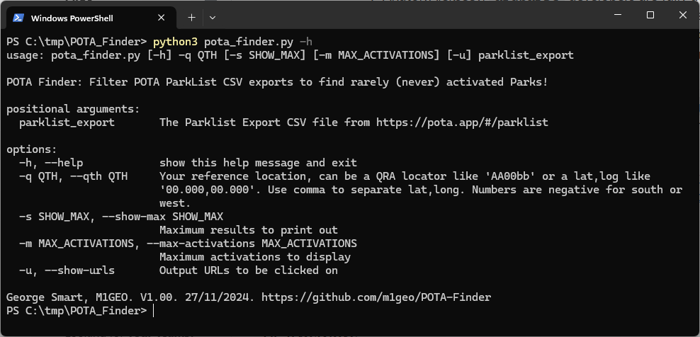
The code can be found on GitHub: https://github.com/m1geo/POTA-Finder. It runs in a command terminal window on any OS that will run Python3. It has a simple help function, and minimal error checking as it was an evening project. The source code should be easy enough to tinker with should you wish to add, change, remove functionality.
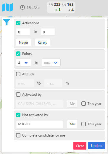
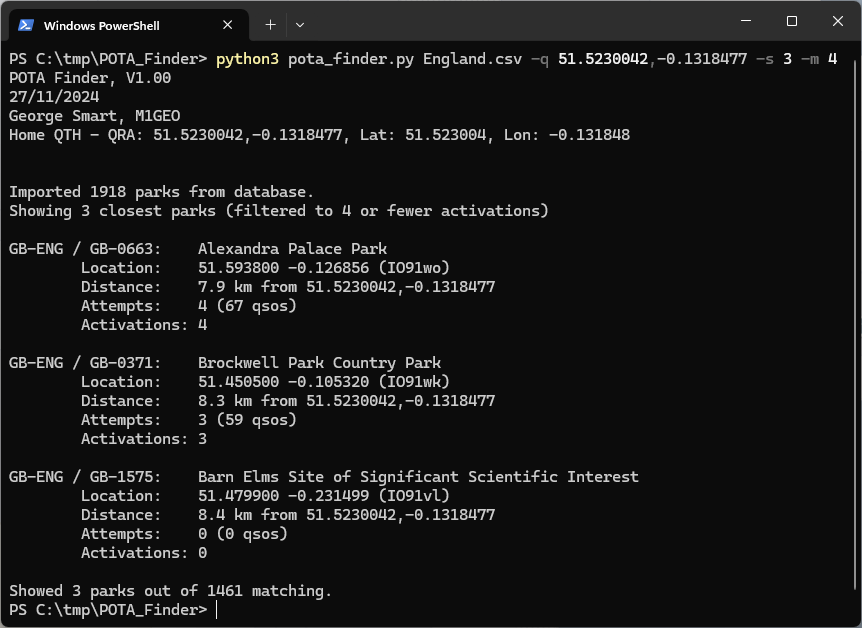
Calling the program with the -h help flag will output the above information to help you get started. You can set the --max-activations to 0 to show unactivated parks, like this:
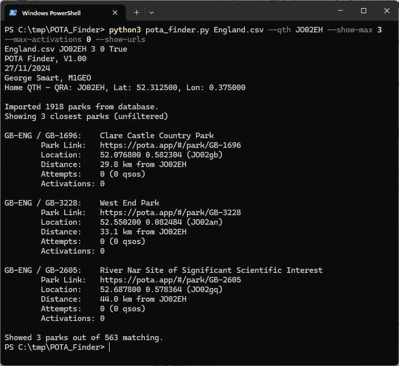
You can also use the shorter command-line options as below, and supply a lat/long as here:
And with that, you can pack your kit in the car and head out for a POTA activation…
As I was unable to take part in the CQWW CW Contest 2020 due to Coronavirus COVID-19 regulations, I decided to experiment with using the wideband SDR of the Hermes Lite 2 SDR (HL2).
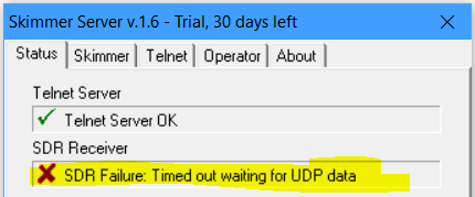
The process appeared to be quite smooth, however upon completion, the CW Skimmer’s Skim Server (SkimSrv) would report that the SDR connection had timed out. This transpired to be the hardware watch dog timer (WDT) timeout inside the FPGA on the Hermes Lite 2 – a precaution to stop the SDR from being stuck in transmit should the connection to it drop:
The solution was two-fold:
Update the HL2 gateware to a version allowing the WDT to be adjusted/disabled
Update the SkimSrv DLL plugin to a version using the WDT configuration
Getting the Latest HL2 Gateware
The gateware of the HL2 is a bit like what you may consider as firmware. Only, firmware is code that runs on a CPU or microcontroller, and gateware is code that configures the internal connections of an FPGA. This difference is immaterial here, but it is useful to know.
There are many versions of gateware available for the Hermes Lite 2. You are best advised to hunt around Steve Haynal KF7O’s project repositories for the Hermes-Lite2 under the gateware\bitfiles folder and find a version that best suits your needs. It is important to note that some of the gateware files in these folders are compiled with special features and are often not recommended for general use. Here I will cover two versions that I find interesting. The first is the standard gateware that supports both transmit and receive on 4 slices. The second receive only gateware swaps the transmit logic for extra receive logic, resulting in 10 receive-only slices.
One final note, the links I provide are for Hermes-Lite 2.0 build5 and later. If you have an earlier build, then there are different files required which are also present in the variants folders.
Standard 4-slice TX/RX gateware
I started off by finding the latest “testing” version of the HL2 gateware, which can be found in the repositories mentioned above. At the time of writing the original article “testing/20201107_72p5” was the latest version that was recommended for more general use. Since the original publication of this post, this has been rolled into the stable/20201212_72p8 release.
Once you have read the readme and are happy with the notes supplied with the version of the bitfile (the actual compiled file the FPGA is sent to configure itself), then you are ready to go.
Use stable/20201212_72p8/hl2b5up_main/hl2b5up_main.rbf (direct link to download) which supports up to 4 receiver slices, but also includes transmit and is suitable for general use – again – read the notes that are supplied! They are important. Whatever you chose, you may need to rename the “.rbf” file to “hl2b5up_main.rbf” to allow it to be flashed by SparkSDR. Quisk doesn’t seem to care what the file is called.
No transmit 10-slice receive gateware
My actual reason for changing the gateware was to try the 10-slice receive gateware for use with SparkSDR as a grabber for CW Skimmer, as well as all of the other digital modes (RTTY, PSK, WSPR, FT8, JT65, etc.).
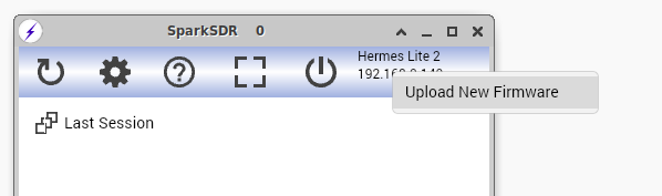
To program the gateware there are two options. I opted to use SparkSDR2 by Alan Hopper M0NNB. The process is easy and SparkSDR2 supports Windows and Linux. Run SparkSDR, press the discovery button (the rotating arrow on the left) until your Hermes Lite 2 is discovered, and then right-click and select firmware. From there, navigate from the downloaded and renamed file “hl2b5up_main.rbf” and press program. It should take around a minute.
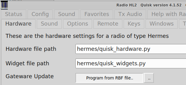
You are also able to use Quisk by James Ahlstrom N2ADR. From the Config dialogue, select your radio, and then select “Program from RBF file”. The update should not take long.
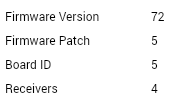
Once the upload is complete, you should power cycle the Hermes Lite 2 SDR, and then check in your favourite program that the update was successful. I checked that the radio still worked, and I could see that the revision gateware had changed to what I expected within SparkSDR: “Version 72 Patch 5” (now superseded by stable 72p8) and that I did indeed have 4 receivers available. If you used a different gateware version, you should see different results here:
Installing the recompiled HermesIntf.dll
Originally, the HermesIntf.dll file was provided by Vasiliy Gokoyev K3IT on the GitHub page HermesIntf. However, this DLL does not take advantage of the extra WDT options available in the HL2 gateware we just updated. To make such updates, this required the original DLL supplied by Vasiliy K3IT to be recompiled, incorporating changes from Steve KF7O’s gateware.
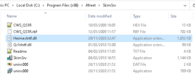
I was beaten to doing this by Robin Davies G7VKQ, who kindly shared the rebuilt DLL file with me on Twitter (thanks!!). This DLL file can be downloaded here: HermesIntf_G7VKQ.zip. There’s also a version by KV4TT (released Jan 2021) which I would suggest using as it has some further tweaks for handling the watchdog timer. This file is then to be copied into the SkimSrv folder, typically located within “C:\Program Files (x86)\Afreet\SkimSrv\” on a modern 64-bit version of Windows. You will of course need to install SkimSrv by Afreet Software from here. A trial version is available – you’ll need the Skim Server, not the standard CW Skimmer.
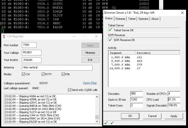
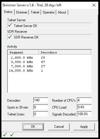
Once you’ve copied the DLL into the installation folder, you are ready to fire-up the SkimSrv. SkimSrv has a little icon in the system tray, as shown below. Click on this to open the SkimSrv settings dialogue.
From here, you can use the Skimmer tab to set up the frequencies, sample rates, radios, etc., to use. This is all as you would expect and is pretty straight forward. Above, you can see I am using the 4 receivers available in the gateware version of the HL2 I chose. The image at the top of the page shows operation during CQWW CW 2020, where there were huge numbers of signals present on the bands.
You can connect a telnet program to “localhost” on port “7300” to connect to the Skimmer Server by default. This acts like a DX Cluster with spotting information.
Uploading to PSKReporter
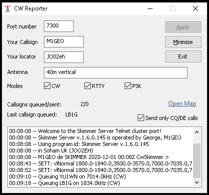
One of the most easy way is use CW Reporter by Philip Gladstone N1DQ. Philip runs PSKReporter, and, offers the CW Reporter application to interface between CW Skimmer Server and PSKReporter. It is easy to set up, working almost out of the box, and translates the DX Cluster style Telnet spots into reports for PSKReporter.info.
One comment to note here is that you should have calibrated your receiver’s frequency before doing this – otherwise, you may be spreading incorrect frequency information.
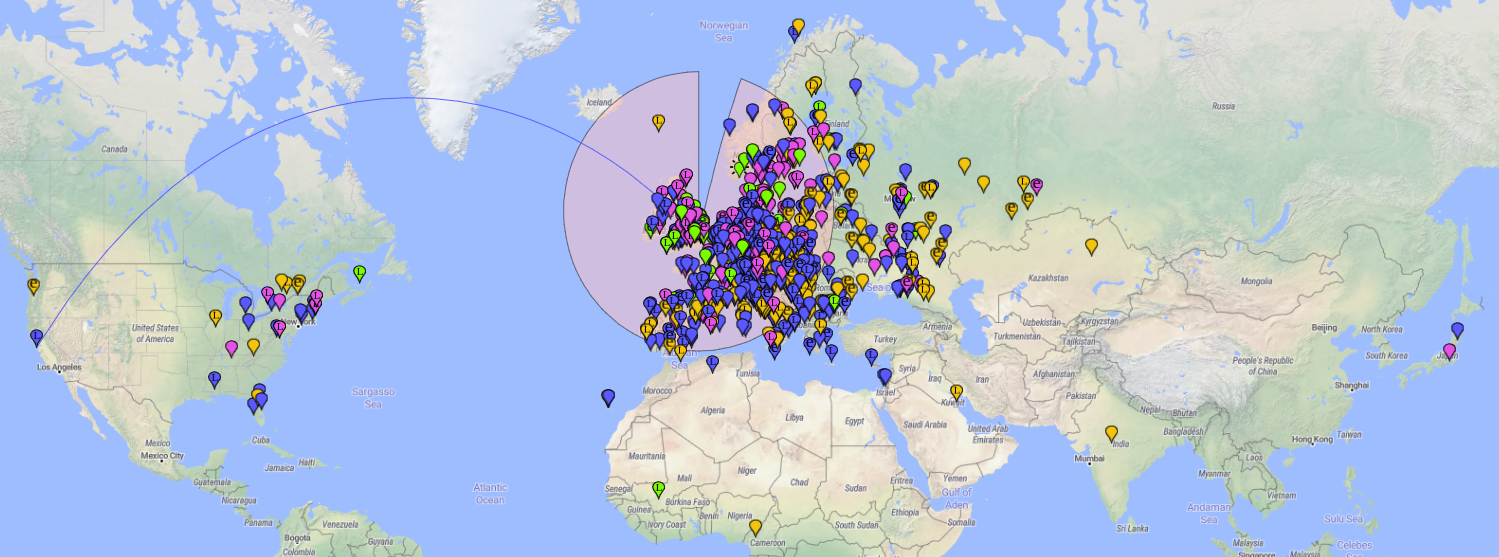
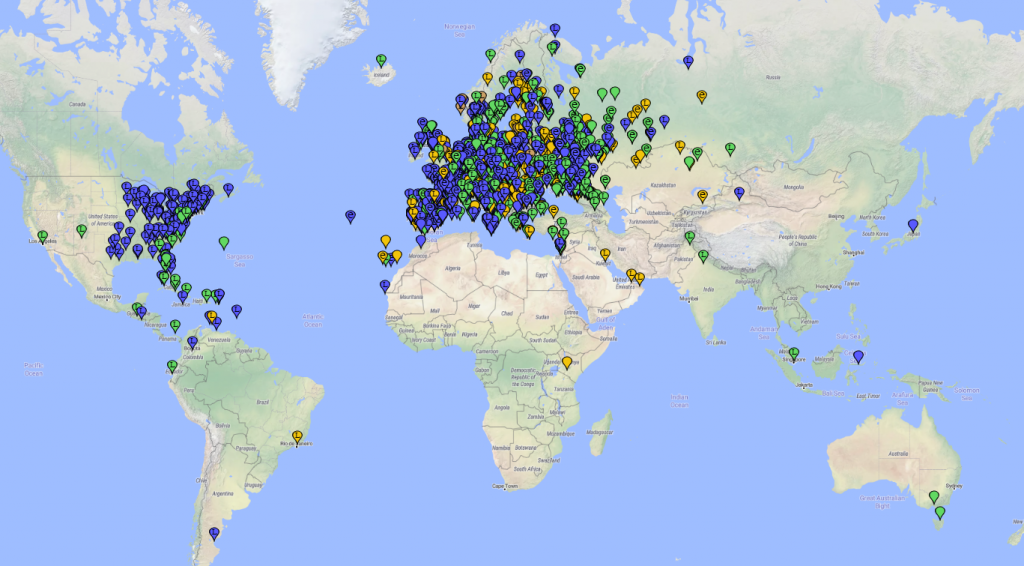
Finally, it is possible to see, on a map, using appropriate filters, what stations I have heard on CW over the past 24 hours:
Click any image to enlarge.
Thanks to everyone who offered help and suggestions along the way!
Recently I purchased a Hermes Lite 2 SDR receiver (HL2 for short), and I am very impressed with it. One of the very nice features is that it lets you receive several chunks of spectrum (“slices” in SDR parlance) at once.
I also found an excellent piece of software for the digital-mode enthusiast called SparkSDR. SparkSDR can make use of the multiple slices offered by HL2, and thus allows for an infinite number of digital mode receivers to be operated using the HL2 slices. SparkSDR also offers the ability to transmit these modes, but for the purposes of this article, I am only concerned with FT8 reception.
Since FT8 came about, the use of WSPR for making test transmissions and observing receiving locations has pretty much died. However, with the widespread update of FT8 (and similar modes such as FT4, etc.) these transmissions may instead be used as transmitting beacons – when a station calls ‘CQ’ (makes a general call soliciting someone to reply), the software sending the FT8 call encodes the senders location (as a QRA locator) into the sent message. A typical CQ may look something like this:
CQ M1GEO JO02
Similarly, the system of another person responding to my CQ call will also encode the distant station’s location, resulting in a response which may look something like this:
M1GEO ZL1A RF72
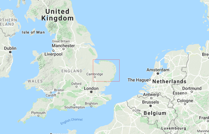
Here “M1GEO” is my callsign, “ZL1A” is a DX (distant) station and “JO02” (and “RF72”) is the first part of the maidenhead locator, covering a 100km square, which looks something like this:
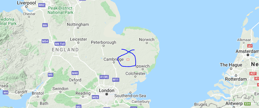
It is possible to use a 6-digit locator, for example JO02HG, which takes the accuracy down to a 10km square (see below). Although there are higher resolution locators than this, they are not often used.
Since we know (at least to within 10km) where a transmitting station is, it becomes possible to plot the stations on a map. You’ve probably seen this done before. Websites like PSKReporter and WSPRnet have been doing this for some time now.
The image above use different coloured markers for different bands:
Marker Colour
Band
Blue
40m (7074 kHz)
Green
30m (10136 kHz)
Yellow
20m (14070 kHz)
Brown
15m (21074 kHz)
I have been recently enjoying the ability to use the same untuned vertical antenna with the same radio on different bands simultaneously (the HL2 lets you remove any band-pass filtering). This allows you to see, for example, that while 40m was good for working Germany, 30m had good propagation into Australia.
PSKReporter lets you filter by mode, band, and time, so you can see what times a given band is open to a specific location. Excellent for helping to fill those missing DXCC slots you may have.
It was interesting for me to see that much of the more remote stations were received on the lower bands, 40 and 30m, and not 20m as I would have expected:
VK7BO at 6:06 UTC on 30m
VK3ZH at 6:33 UTC on 30m
K6SY at 5:28 UTC on 30m
LU1WFU at 1:50 UTC on 40m
YE8QR at 14:46 UTC on 40m
Although at the time of writing (August 2020), HF conditions are quite poor, not all of the lack of performance on 20m can be explained due to the band conditions, since 20m is still open to South America and into Asia.
Animating the propagation
After looking at these static images, I wanted to see how things changed with time. Could I, for example, see when the best time to work the west cost of the USA would be? I decided to make a time-lapse animation. The animation runs for approximately 3 days, and includes the following FT8 decodes:
Band
Decodes
40m (7074 kHz)
72,404
30m (10136 kHz)
33,871
20m (14070 kHz)
156,636
15m (21074 kHz)
3,453
It is clear to see sudden bursts of colour when a band opens, and to watch conditions change throughout the day. The dates here were for a Friday to Monday, so, there’s plenty of weekend activity.
I’m keen to further explore the possibilities of this.
I noticed after a while, that my BER percentage of my MMDVM_HS_Hat and Pi-Star setup was significantly higher than other users, at around 3.5%. I know from setting up GB7KH that getting this correct takes patience. I also happen to know that the design of the MMDVM_HS_Hat uses inexpensive TCXOs to provide frequency and timing references. As such, some calibration can do wonders for the BER on DMR.
For this mini-guide, I shall use my TYT MD-380 handheld DMR radio. My hotspot is set to use a nominal frequency of 434.250 MHz as the carrier frequency.
Using the DMR handheld as a transmitter on low power, it should be possible to better match the frequency of the receiver to the transmitter – this process isn’t ideal, because it could equally be the handheld frequency which is incorrect – but at least they’ll match.
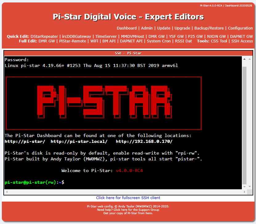
We’ll need to get SSH access to the underlying Linux system on the Pi-Star. You can either use the “SSH Access” tab from the Pi-Star Expert menu, as below:
Pi-Star SSH Access via Expert menu
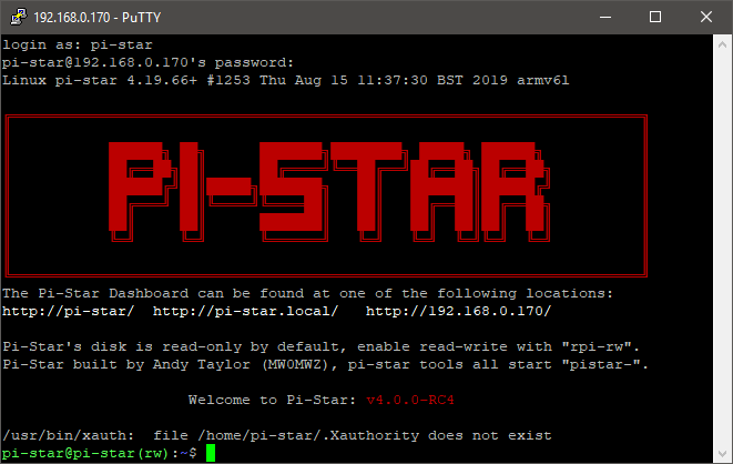
Or you may prefer to SSH into the Pi-Star with your preferred SSH client – I use PuTTY. Either option will work here.
The program we need is called MMDVMCal. Fortunately, there’s a version compiled for us already in Pi-Star. From the Pi-Star console terminal, the following command will start the MMDVMCal program where we’ll do our testing:
$ sudo pistar-mmdvmcal
Using MMDVMCal
When the program starts, you’re greeted with the following command line instructions. You may also see some debug/warnings about
Starting Calibration… Version: 1, description: MMDVM_HS_Hat-v1.4.17 20190529 14.7456MHz ADF7021 FW by CA6JAU GitID #cc451c4 The commands are: H/h Display help Q/q Quit W/w Enable/disable modem debug messages E/e Enter frequency (current: 433000000 Hz) F Increase frequency f Decrease frequency Z/z Enter frequency step T Increase deviation t Decrease deviation P Increase RF power p Decrease RF power C/c Carrier Only Mode K/k Set FM Deviation Modes D/d DMR Deviation Mode (Adjust for 2.75Khz Deviation) M/m DMR Simplex 1031 Hz Test Pattern (CC1 ID1 TG9) K/k BER Test Mode (FEC) for D-Star b BER Test Mode (FEC) for DMR Simplex (CC1) B BER Test Mode (1031 Hz Test Pattern) for DMR Simplex (CC1 ID1 TG9) J BER Test Mode (FEC) for YSF j BER Test Mode (FEC) for P25 n BER Test Mode (FEC) for NXDN g POCSAG 600Hz Test Pattern S/s RSSI Mode I/i Interrupt Counter Mode V/v Display version of MMDVMCal <space> Toggle transmit
The first thing to do is to set the MMDVMCal frequency. I did this by pressing “E” followed by the frequency of my radio (434.250 MHz) in Hz.
e
434250000
You should see this frequency echoed back in brackets once the menu is reprinted to the screen. If you look at the example above, you’ll see that the frequency is 433000000 Hz (or 433.000 MHz). Pressing “b” will enter “BER Test Mode (FEC) for DMR Simplex” mode:
b
At this point, a quick transmission will show the exact BER:
DMR voice header received DMR voice header received DMR voice header received DMR audio seq. 0, FEC BER % (errs): 2.837% (4/141) DMR audio seq. 1, FEC BER % (errs): 2.837% (4/141) DMR audio seq. 2, FEC BER % (errs): 3.546% (5/141) DMR audio seq. 3, FEC BER % (errs): 1.418% (2/141) DMR audio seq. 4, FEC BER % (errs): 0.709% (1/141) DMR audio seq. 5, FEC BER % (errs): 2.128% (3/141) DMR voice end received, total frames: 6, bits: 846, errors: 19, BER: 2.2459%
My BER is showing as 2.5%. Not awful, but with some room for improvement.
The process of finding the ‘perfect’ value is twofold. The first is to find the approximate frequency, and then dial in the exact value. Here, we’re trying to find out the difference between the nominal frequency (in my case 434.250 MHz) and the optimal working frequency.
From the menu above, you’ll note that both “F” and “f” (both upper and lower case) increase and decrease the frequency respectively. By holding your radio in transmit, repeatedly press the F key until you the MMDVM_HS_Hat looses the transmission from your handheld. You’ll see the TX frequency announced with each change of frequency – allow time between each step (around 10 seconds on each frequency).
Keep going in one direction until the software reports “Transmission Lost” – note the final frequency down. You can see this by pressing “H” or “h” to reprint the menu. For me, the first limit I reached was 434249800 Hz by repeatedly pressing “f” to lower the frequency.
From here, you can find the mean (centre) frequency: (434249800 + 434250800)/2 = 434250300 Hz (300Hz higher than the nominal).
Use the “E” command once again and enter your new mean frequency – for me, this was 434250300 Hz.
e
434250300
You can then either enter frequencies yourself stepping 10 Hz at a time until you find the frequency yielding the best BER, or you can use the “Z” and “z” commands to increase or decrease the steps, and continue using the “F” and “f” commands to ‘home in’ on the value. I tabulated my results to give me a clear understanding of what was going on. I first went with 25 Hz steps (half the default 50 Hz steps) and found the following values for a 15 second transmission on each frequency. At the end of each transmission, status (including BER) are reported. You can see that the optimum value was very close to my mean value.
You can see that the optimum value was very close to my mean value. I experimented with even smaller steps, but didn’t really improve much on the 0.1% BER. This value is definitely good enough, and is an order of magnitude better than what I had previously!
Since I also use D-STAR, I quickly pressed “K” to enter D-STAR BER test mode, and, with the best settings from DMR, I keyed my Kenwood TH-D74 handheld – everything was fine here, too:
D-Star audio FEC BER % (errs): 0.000% (0/48) D-Star audio FEC BER % (errs): 0.000% (0/48) D-Star audio FEC BER % (errs): 0.000% (0/48) D-Star audio FEC BER % (errs): 0.000% (0/48) D-Star audio FEC BER % (errs): 0.000% (0/48) D-Star audio FEC BER % (errs): 0.000% (0/48) D-Star voice end received, total frames: 214, bits: 10272, errors: 0, BER: 0.00000%
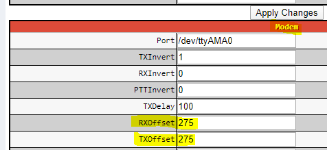
Taking the frequency for your lowest BER (in my case 434250275 Hz), the offset is easy to calculate: Simply subtract the best BER frequency from the nominal frequency to find the offset: 434250275 – 434250000 = 275 Hz (note, this can be negative).
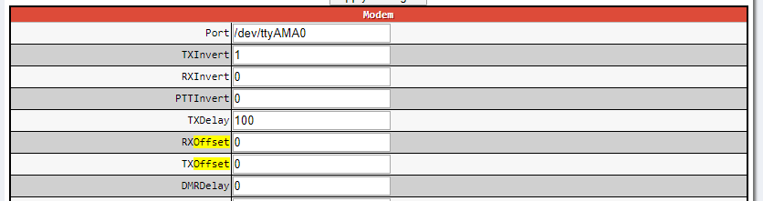
Applying the Offset
We next need to apply our offset (in my case +275 Hz) to the main MMDVMHost application running on the Pi-Star. This is done through the expert configuration.
Inside the Pi-Star configuration, head to the Admin Expert menu once again and select MMDVMHost.
Inserting our calculated offset (in Hertz) from the above.
This page assumes some basic familiarity with Linux. It assumes a clean install of Ubuntu 18.04 and installs Eclipse Photon. I install the CPP version, but you’re free to choose when the option presents itself!
Update the OS
First thing to do is to update the operating system. This is easily achieved by running the following two commands:
sudo apt update
sudo apt upgrade
These commands may take a while to complete, depending on what there is to update and how fast your internet connection is.
Installing Java Development Kit (JDK) 8
Since Eclipse is written in Java, we will need the latest version. I’m not sure if the Java Runtime Environment (JRE) alone is enough, but I have installed the full JDK anyway.
Firstly we add the third party JDK PPA repository and update the package manger index
sudo add-apt-repository ppa:webupd8team/java
sudo apt update
Next we must actually install the JDK:
sudo apt install oracle-java8-installer
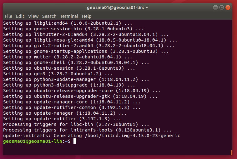
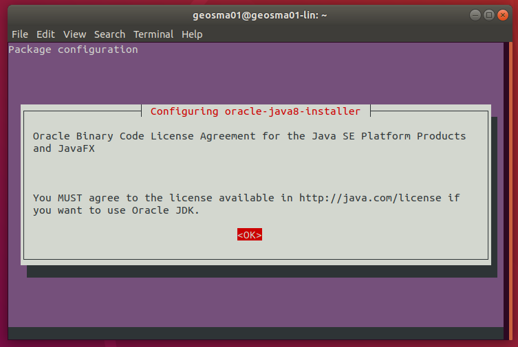
This will pull in a few extra packages, such as java-common, oracle-java8-set-default (which makes sure that this installed version of Java is the system default), font packages and so on. You’ll be guided through the Java 8 installation with an ncurses based installer:
You must accept the Oracle Binary Code licence. The download for Java 8-1u171 was 182 MB. To confirm the installer completed correctly, scroll up in the terminal window. You should see something explaining that the installation finished successfully. To confirm this, and check the version installed, you can run the following from the terminal:
javac -version
javac 1.8.0_171 [or similar result expected]
Installing Eclipse
The Eclipse installer can be found on the Eclipse project download page: https://www.eclipse.org/downloads/. At the time of writing, the Eclipse Photon installer was 45.9 MB. I downloaded it using the Mozilla Firefox browser, and saved the installer into my user’s download folder (/home/geosma01/Downloads/).
Once downloaded, switch back to your terminal program, and change directory into the downloads folder and extract the downloaded TAR/GZIP archive and change directory into it:
cd ~/Downloads/
tar xvfz eclipse-inst-linux64.tar.gz
We’re now ready to run the installer. If we change into the newly extracted folder and then run the installer, we should be good to go:
cd eclipse-installer
./eclipse-inst
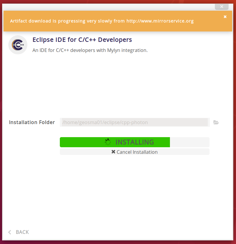
I ran into trouble installing Eclipse as root, so I install it into my own user space: ~/eclipse/cpp-photon
Accept any licences it prompts for:
Once the installer has finished, you can start Eclipse by pressing Launch. We’ll make a desktop shortcut in a few moments…
And eventually…
Now we have Eclipse running, we should get ourselves an icon to easily start it.
Creating a Menu Icon
Next we will create a menu shortcut. We will create this using a basic terminal-based text editor (nano). Running the following will open the file:
nano ~/.local/share/applications/eclipse.desktop
Then, copy and paste the following, as you see appropriate – you should change my username (geosma01) to your own at the very least:
If all has gone well, you’ll see something like the following inside the menu:
Installing PyDev
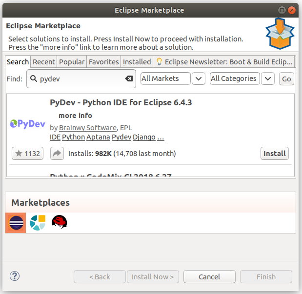
PyDev can be easily installed through the Eclipse Marketplace. From inside Eclipse, click Help on the menu, and select Eclipse Marketplace. You should be presented with the following window. You can then enter “pydev” into the search, and then click Install on the entry shown below:
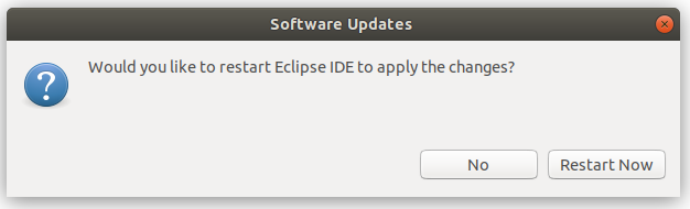
Confirm your selections, accept the licence conditions, and you’re good to go! Once installed, click on Restart Now and you’re done!
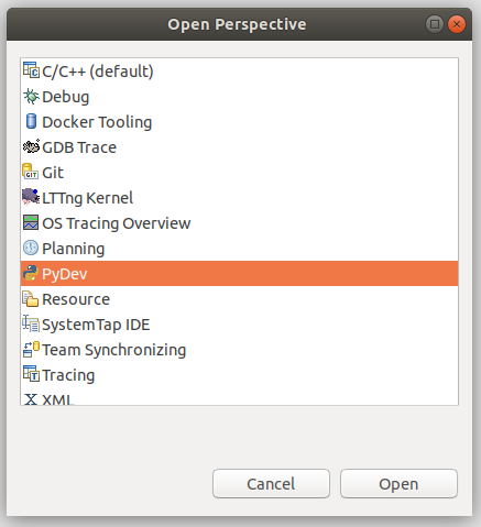
Once restarted, you can open a PyDev Perspective by selecting Window from the menu, selecting Perspective > Open Perspective > Other and selecting PyDev:
You’re ready to go!
An online scrapbook full of half-baked projects and silly ideas.